Line charts to emphasize changes in the dependent variable

Let’s pick a series of population data taken from the Spanish Labor Force Survey:

library(tidyverse) #to load ggplot and dplyr
library(ESdata)    #to get the data
pop_quarterly <- epa_edad %>% 
  filter(region=="ES", edad=="total", sexo=="total", dato=="pob")
pop_quarterly

## # A tibble: 75 x 6
##    periodo    region edad  sexo  dato   valor
##    <date>     <chr>  <chr> <chr> <chr>  <dbl>
##  1 2020-09-30 ES     total total pob   46904.
##  2 2020-06-30 ES     total total pob   46896.
##  3 2020-01-31 ES     total total pob   46874.
##  4 2019-12-31 ES     total total pob   46794.
##  5 2019-09-30 ES     total total pob   46702.
##  6 2019-06-30 ES     total total pob   46599 
##  7 2019-01-31 ES     total total pob   46523.
##  8 2018-12-31 ES     total total pob   46435.
##  9 2018-09-30 ES     total total pob   46326.
## 10 2018-06-30 ES     total total pob   46241 
## # … with 65 more rows

pop_quarterly is a data frame with 75 observations. e will plot the independent variable periodo (in Date format) in the horizontal axis, and the dependent variable valor in the vertical axis, so that the aesthetic is aes(periodo, valor).

We use geom_line() to plot line charts to emphasize changes of the dependent variable as the independent variable changes. ggplot is building by default a vertical axis that does not start from zero, following Bergstrom and West’s recommendations. I have changed axis names and presented a title with labs, and changed the default theme to theme_bw().

pop_quarterly %>%
  ggplot(aes(periodo, valor)) +
  geom_line() +
  labs(title="Evolution of Spanish population", x="", y="population (thousands)") +
  theme_bw()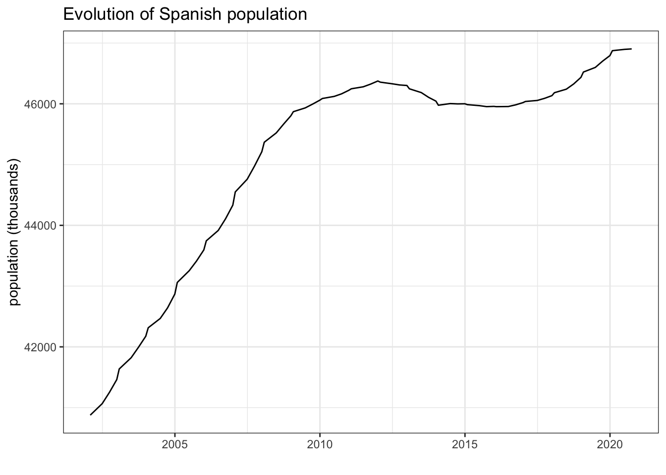

We observe Spanish population increased steadily from 2004 to approximately 2012, and that has started recovering by 2017 but with a slower pace than the previous growth cycle. Vertical axis ranges between 41 and 46 million people, which is the variation of population for this temporal series.

We are now interested in analyzing the evolution of Spanish population by gender. We need a dataset including the value of male and female Spanish population for each observation:

pop_quarterly_gender <- epa_edad %>% 
  filter(region=="ES", edad=="total", sexo!="total", dato=="pob")
pop_quarterly_gender

## # A tibble: 150 x 6
##    periodo    region edad  sexo    dato   valor
##    <date>     <chr>  <chr> <chr>   <chr>  <dbl>
##  1 2020-09-30 ES     total hombres pob   23016.
##  2 2020-06-30 ES     total hombres pob   23013.
##  3 2020-01-31 ES     total hombres pob   23004.
##  4 2019-12-31 ES     total hombres pob   22966 
##  5 2019-09-30 ES     total hombres pob   22924.
##  6 2019-06-30 ES     total hombres pob   22874.
##  7 2019-01-31 ES     total hombres pob   22836.
##  8 2018-12-31 ES     total hombres pob   22792.
##  9 2018-09-30 ES     total hombres pob   22740.
## 10 2018-06-30 ES     total hombres pob   22699.
## # … with 140 more rows

The pop_quarterly_gender data frame has 150, twice the rows of the previous table. This is a dataset in long format, and it is tidy data because each row represents an observation. Remember that tidyverse functions expect tidy data to work.

By adding a color parameter to the aesthetic, ggplot will plot a line for each category. The value of color should be the variable defining the level of the categorical variable for each observation, which here is sexo. Now the aesthetic is aes(periodo, valor, color=sexo).

By introducing the colorin the aesthetic, we are not defining the colors, but defining what is the use of the color in the plot. To override ggplot defaults I have used scale_color_manual to change the legend title, the value of labels for each level of the categorical variable and the color of each line. I have used theme(legend.position = "bottom") to put the legend at the bottom of the plot, so that the chart can be seen larger than in the default legend position at the right.

pop_quarterly_gender %>%
  ggplot(aes(periodo, valor, color=sexo)) +
  geom_line() +
  labs(title="Evolution of Spanish population by gender", x="", y="population (thousands)") +
  scale_color_manual(name="gender", labels=c("men", "women"), values =c("#0066CC", "#CC0000")) +
  theme_bw() +
  theme(legend.position = "bottom")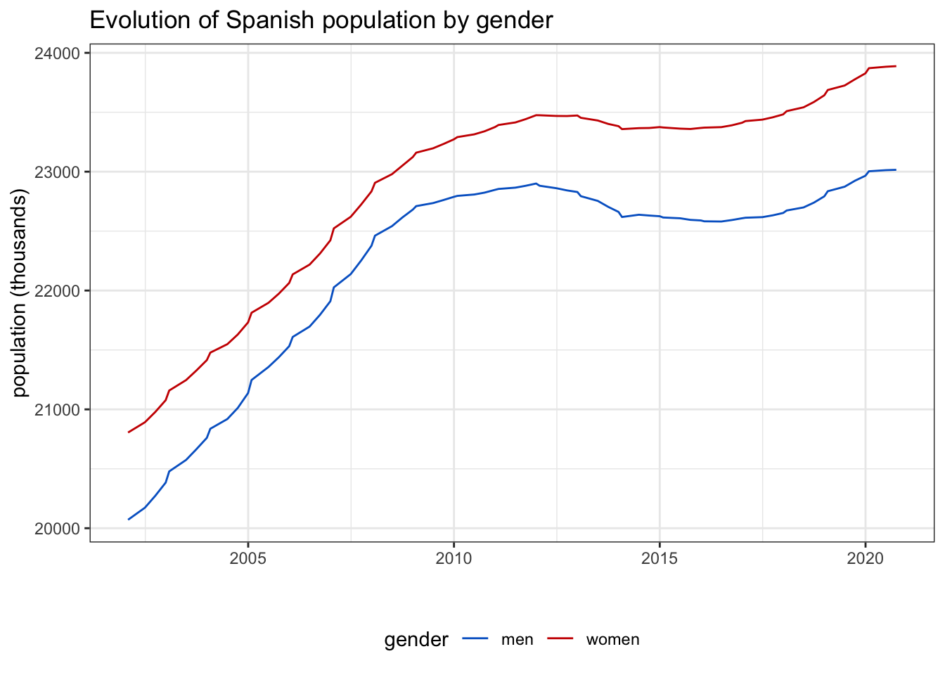

In this line chart we observe that there are consistently more women than men living in Spain, and that the decrease of population has been slightly larger for men than for women.

Bar charts to emphasize absolute magnitude of the dependent variable

Let’s examine now the evolution of absolute values of Spanish population. Instead of quarterly data, we will use a yearly dataset including the last observation of each year:

library(lubridate) #to get the year of each observation
pop_yearly <- epa_edad %>% 
  filter(region=="ES", edad=="total", sexo=="total", dato=="pob") %>%
  mutate(year=year(periodo)) %>%
  group_by(year) %>%
  summarise(pop = last(valor), .groups = "drop")
pop_yearly

## # A tibble: 19 x 2
##     year    pop
##    <dbl>  <dbl>
##  1  2002 40876.
##  2  2003 41636.
##  3  2004 42314.
##  4  2005 43060.
##  5  2006 43745 
##  6  2007 44550.
##  7  2008 45368.
##  8  2009 45870.
##  9  2010 46087.
## 10  2011 46248.
## 11  2012 46356.
## 12  2013 46247.
## 13  2014 45977.
## 14  2015 45986.
## 15  2016 45953.
## 16  2017 46038.
## 17  2018 46183.
## 18  2019 46523.
## 19  2020 46874.

To examinethe absolute magnitude of the dependent variable, we build a bar plot using geom_col(). I have used labs and theme_bw() like in the previous plots and changed the color of the bars for aesthetic reasons with the fill parameter.

pop_yearly %>% 
  ggplot(aes(year, pop)) +
  geom_col(fill="#808080") +
  labs(title="Evolution of Spanish population", x="", y="population (thousands)") +
  theme_bw()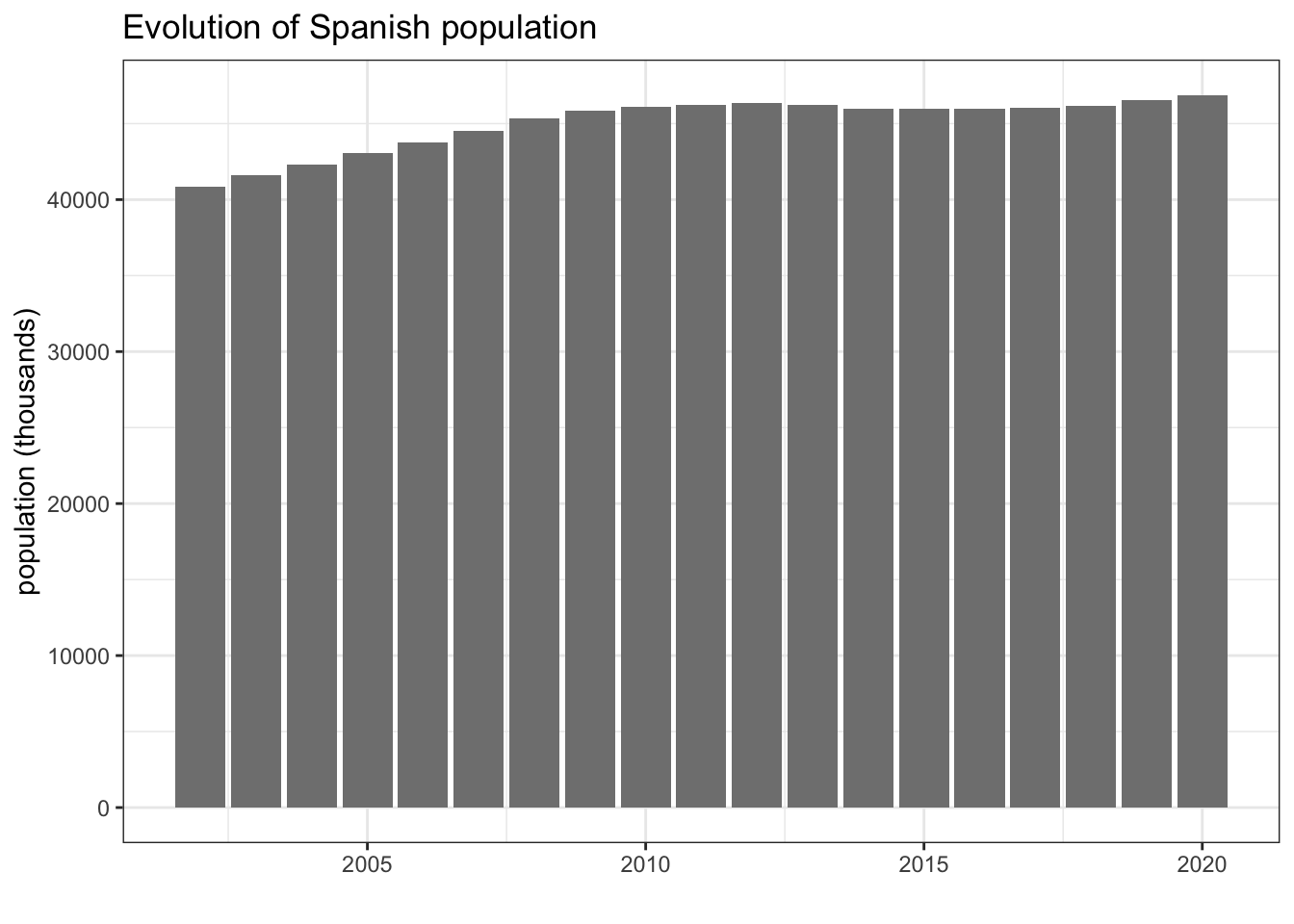

With this bar plot, we focus on absolute magnitudes so we put changes in perspective. We realize that the variations of total population are relatively small respect to the total population.

Let’s examine the yearly evolution of Spanish population by gender, building the adequate dataset in long format:

pop_yearly_gender <- epa_edad %>% 
  filter(region=="ES", edad=="total", sexo!="total", dato=="pob") %>%
  mutate(year=year(periodo)) %>%
  group_by(year, sexo) %>%
  summarise(pop = last(valor), .groups = "drop")
pop_yearly_gender

## # A tibble: 38 x 3
##     year sexo       pop
##    <dbl> <chr>    <dbl>
##  1  2002 hombres 20071 
##  2  2002 mujeres 20805.
##  3  2003 hombres 20478 
##  4  2003 mujeres 21158.
##  5  2004 hombres 20837.
##  6  2004 mujeres 21478.
##  7  2005 hombres 21247.
##  8  2005 mujeres 21813.
##  9  2006 hombres 21609.
## 10  2006 mujeres 22136.
## # … with 28 more rows

To distinguish by gender, I have added fill to the aesthetic, and I have used scale_fill_manual to customize the plot. I have chosen now slightly paler shades of blue and red for aesthetic convenience.

pop_yearly_gender %>%
  ggplot(aes(year, pop, fill=sexo)) +
  geom_col() +
  labs(title="Evolution of Spanish population by gender", x="", y="population (thousands)") +
  scale_fill_manual(name="gender", labels=c("men", "women"), values =c("#3399FF", "#FF3333")) +
  theme_bw() +
  theme(legend.position = "bottom")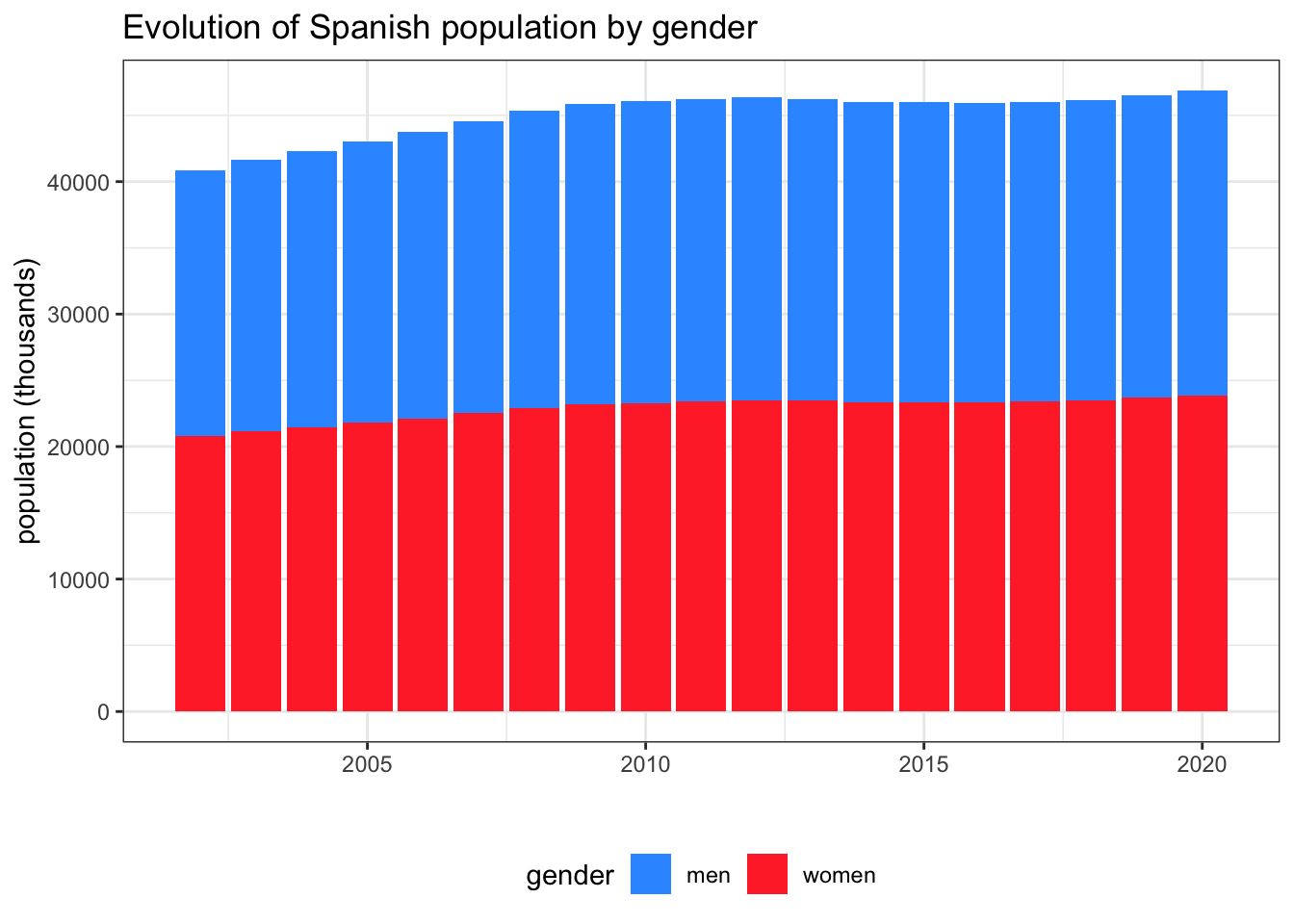

In this barplot bars are stacked, meaning that we have a bar for each year with two colors, one for each category. This representation is adequate here, because the sum of both categories accounts for the total population. If we want to compare the values for each category in each year plotting bars for each category side by side, we can specify position = "dodge" inside geom_col():

pop_yearly_gender %>%
  ggplot(aes(year, pop, fill=sexo)) +
  geom_col(position = "dodge") +
  labs(title="Evolution of Spanish population by gender", x="", y="population (thousands)") +
  scale_fill_manual(name="gender", labels=c("men", "women"), values =c("#3399FF", "#FF3333")) +
  theme_bw() +
  theme(legend.position = "bottom")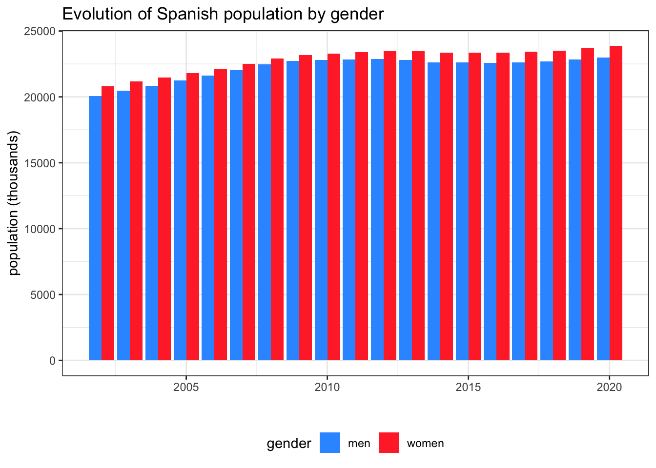

Area charts to emphasize the absolute magnitude of the depedent variable

To build the column plots, we have picked an observation for each year, as a bar plot with quarterly values has too many bars to visualize them correctly. An alternative to visualize absolute magnitude of a dependent variable with many observations is geom_area(). Let’s examine the absolute magnitude of men and women population with an area plot:

pop_quarterly_gender %>%
  ggplot(aes(periodo, valor, fill=sexo)) +
  geom_area() +
  labs(title="Evolution of Spanish population by gender", x="", y="population (thousands)") +
  scale_fill_manual(name="gender", labels=c("men", "women"), values =c("#3399FF", "#FF3333")) +
  theme_bw() +
  theme(legend.position = "bottom")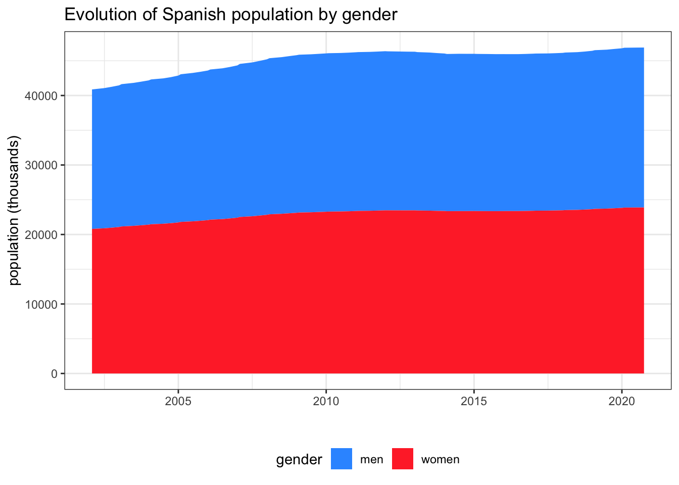

We have used geom_area() to examine the absolute magnitude of temporal evolution of population with pop_quarterly_gender, introducing fill in the aesthetic.

Examining relationships between dependent and independent variables

Whenever we are examining the relationship between two variables, the first thing we need to ask ourselves is if there is an evident dependence relatiosnship between them If there is not, it may be adequate to use a scatterplot to represent them. If the dependence relationship exists, the representation to choose will depend on our intentions:

• If we intend to examine changes of the dependent variable, we will use line plots. We can do that with geom_line() and examine different levels of a categorical variable including color in the aesthetic.
• If we want to examine the absolute magnitude of the dependent variable we will use bar plots with geom_col(), or area plots with geom_area(). In these plots, we use fill to examine the evolution of different levels of a categorical variable.

In both cases, ggplot will set by default the adequate range of values for the vertical axis. In line plots, vertical axis will be set to the range of values where change takes place. In bar and area plots, the vertical axis will start from zero.

Reference

Bergstrm, Carl T. & West, Jevin D. (2020). Calling bullshit: The art of skepticism in a data-driven world. Random House, New York.