In a previous post I presented a small binary classification problem, consisting in finding if an observation of the iris dataset belongs to the versicolor species. Remember that the target variable must be a factor, with first level associated to the positive case:
iris <- iris |>
  mutate(is_versicolor = ifelse(Species == "versicolor", "versicolor", "not_versicolor")) |>
  mutate(is_versicolor =factor(is_versicolor, levels = c("versicolor", "not_versicolor")))
The recipe of this problem is straightforward: remove correlated predictors, and normalize (centering and scaling) the remaining predictors:
iris_recipe <- iris |>
  recipe(is_versicolor ~.) |>
  step_rm(Species) |>
  step_corr(all_predictors()) |>
  step_normalize(all_predictors(), -all_outcomes())
Here I will introduce the receiver operating characteristic (ROC) curve in the context of performance assessment of classification problems. We’ll assess the performance of two predictive models with the ROC curve, and then examine the performance of a bad classifier with the same metric.
Logistic Regression
Let’s begin fitting a logistic regression model:
lr <- logistic_reg() |>
  set_engine("glm")

iris_lr_wf <- workflow() |>
  add_recipe(iris_recipe) |>
  add_model(lr)
With predict(iris) we predict the class of each observation:
iris_pred_lr <- iris_lr_wf |>
  fit(iris) |>
  predict(iris)
iris_pred_lr
## # A tibble: 150 × 1
## .pred_class
## <fct>
## 1 not_versicolor
## 2 not_versicolor
## 3 not_versicolor
## 4 not_versicolor
## 5 not_versicolor
## 6 not_versicolor
## 7 not_versicolor
## 8 not_versicolor
## 9 not_versicolor
## 10 not_versicolor
## # … with 140 more rowsIn logistic regression, the class of each observation is assigned using its probability to belong to each class. This probability is used to construct the ROC curve, and we can obtain it using predict with type = "prob":
iris_prob_lr <- iris_lr_wf |>
  fit(iris) |>
  predict(iris, type = "prob")
iris_prob_lr
## # A tibble: 150 × 2
## .pred_versicolor .pred_not_versicolor
## <dbl> <dbl>
## 1 0.0977 0.902
## 2 0.364 0.636
## 3 0.195 0.805
## 4 0.245 0.755
## 5 0.0658 0.934
## 6 0.0259 0.974
## 7 0.0914 0.909
## 8 0.127 0.873
## 9 0.367 0.633
## 10 0.303 0.697
## # … with 140 more rowsLet’s bind the outcomes with the original dataset:
iris_lr <- bind_cols(iris, iris_pred_lr, iris_prob_lr)Random Forests
Let’s replicate the same workflow with random forests:
rf <- rand_forest(mode = "classification", trees = 100) |>
  set_engine("ranger")

iris_rf_wf <- workflow() |>
  add_recipe(iris_recipe) |>
  add_model(rf)

iris_pred_rf <- iris_rf_wf |>
  fit(iris) |>
  predict(iris)

iris_prob_rf <- iris_rf_wf |>
  fit(iris) |>
  predict(iris, type = "prob")

iris_rf <- bind_cols(iris, iris_pred_rf, iris_prob_rf)
The ROC Curve
To classify an observation as positive or negative class from probabilities we need a threshold value, a value between 0 and 1 so that:
- If observation’s probability of belonging to positive class is below the threshold the observation is labelled as negative.
- If observation’s probability of belonging to positive class is above the threshold the observation is labelled as positive.
In a ROC curve we plot two performance metrics:
- On the x axis we plot 1 - specificity, the ratio of negative observations classified correctly.
- On the x axis we plot sensitivity, the ratio of positive observations classified correctly.
In the ROC curve, each point is the value of sensitivity and 1 - specificity for a specific threshold value. The ROC curve allows us to assess the balance between sensitivity and specificity of a classifier.
We will always have two points in every ROC curve:
- If threshold = 1, all observations are classified as negative. Sensitivity is equal to 0 and specificity is equal to 1. This is the (0, 0) point of the ROC curve.
- If threshold = 0, all observations are classified as positive. Sensitivity is equal to 1 and specificity is equal to 0. This is the (1, 1) point of the ROC curve.
A perfect classifier has sensitivity and specificity equal to one, which corresponds with the (0, 1) point in the ROC curve.
roc_df <- data.frame(x_roc = c(0,0,1),
                     y_roc = c(0,1,1),
                     threshold = c("threshold=1", "perfect class.", "threshold=0"))

ggplot(roc_df, aes(x_roc,y_roc, label=threshold)) +
  geom_point(size=2) +
  xlim(-0.1, 1.1) +
  ylim(0, 1.1) +
  geom_text(vjust=0, nudge_y = 0.05) +
  geom_abline(slope=1, intercept = 0, linetype = "dashed", size=0.2) +
  theme_bw() +
  labs(x="1-specificity", y="sensitivity")
## Warning: Using `size` aesthetic for lines was deprecated in ggplot2 3.4.0.
## ℹ Please use `linewidth` instead.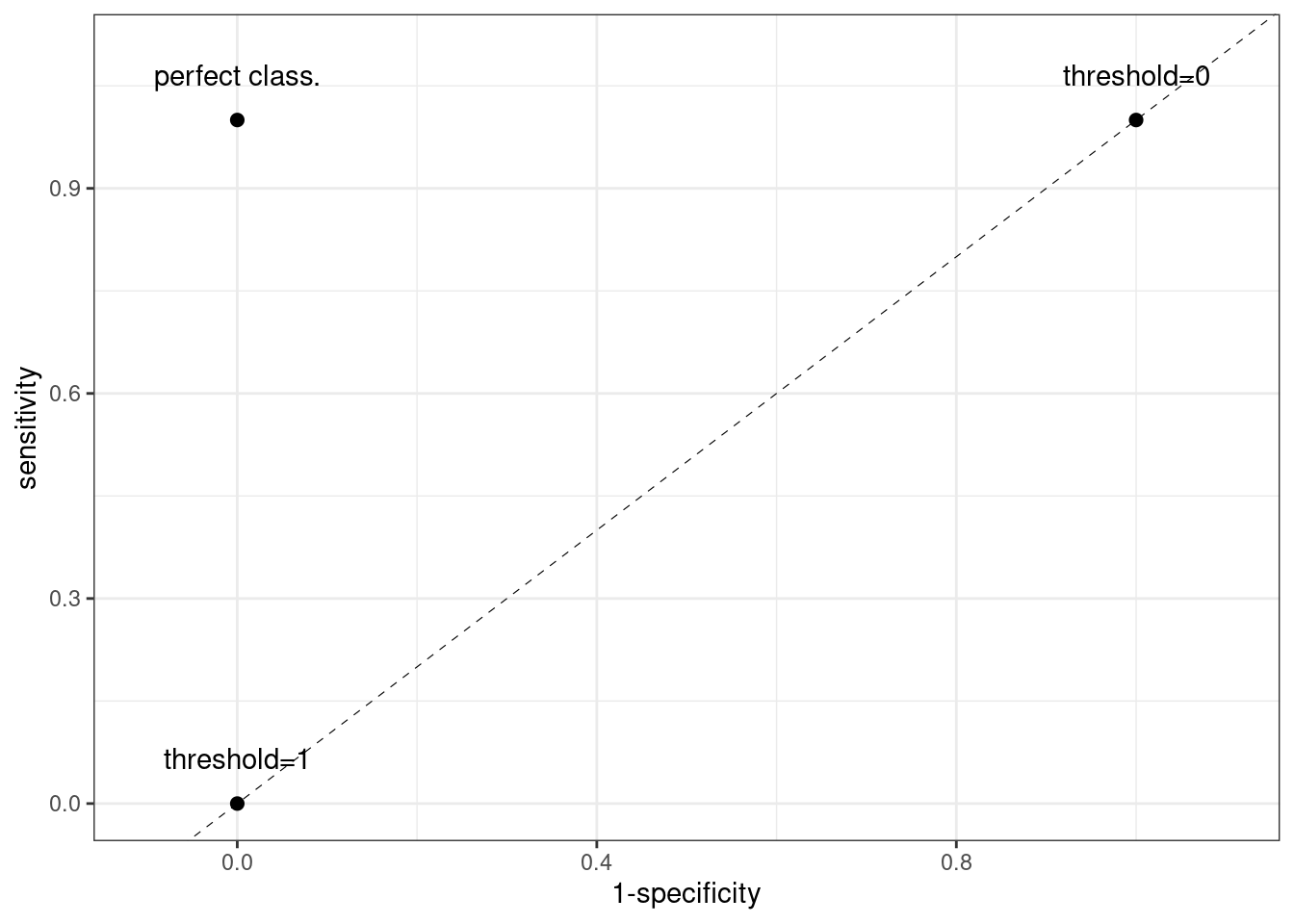
This curve can be turned into a number with the area under the ROC curve (AUC). This area will be a value between 1 and 0.5, being 1 the value of a perfect classifier. A classifier with ana AUC below 0.5 can be transformed into a better predictor just reversing the outcome (classifying positives as negatives and vice versa).
Let’s see the performance of logistic regression and random forests using the ROC curve.
ROC Curve for Logistic Regression
Here is a plot of the ROC curve for logistic regression. The points in red correspond with threshold values around 0.5, the usual cutoff values when predicting classes.
roc_curve_lr <- iris_lr |>
  roc_curve(truth = is_versicolor, estimate = .pred_versicolor) |>
  mutate(x_roc = 1-sensitivity, y_roc=specificity)

sens_spec_lr <- roc_curve_lr |>
  filter(.threshold > 0.48, .threshold < 0.52)

roc_curve_lr |>
  ggplot(aes(x_roc, y_roc)) +
  geom_point(size=0.5)  +
  geom_point(data=sens_spec_lr, aes(x_roc, y_roc), size = 3, color = "red") +
  geom_line(size=0.3) +
  geom_abline(slope=1, intercept = 0, linetype = "dashed", size=0.2) +
  theme_bw() +
  labs(x="1-specificity", y="sensitivity")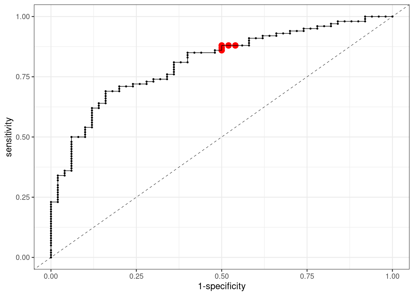
We can obtain the ROC curve faster in tidymodels doing:
iris_lr |>
  roc_curve(truth = is_versicolor, estimate = .pred_versicolor) |>
  autoplot()
The AUC is equal to:
iris_lr |>
  roc_auc(is_versicolor, .pred_versicolor)
## # A tibble: 1 × 3
## .metric .estimator .estimate
## <chr> <chr> <dbl>
## 1 roc_auc binary 0.809Examiing the ROC and the AUC we observe that the performance of logistic regression is relatively poor. Let’s compare it with random forests.
ROC Curve for Random Forests
This is the ROC curve for random forests. This curve is close to a perfect classifier:
roc_curve_rf <- iris_rf |>
  roc_curve(truth = is_versicolor, estimate = .pred_versicolor) |>
  mutate(x_roc = 1-sensitivity, y_roc=specificity)

sens_spec_rf <- roc_curve_rf |>
  filter(.threshold > 0.4, .threshold < 0.6)

roc_curve_rf |>
  ggplot(aes(x_roc, y_roc)) +
  geom_point(size=0.5)  +
  geom_point(data=sens_spec_rf, aes(x_roc, y_roc), size = 3, color = "red") +
  geom_line(size=0.3) +
  geom_abline(slope=1, intercept = 0, linetype = "dashed", size=0.2) +
  theme_bw() +
  labs(x="1-specificity", y="sensitivity")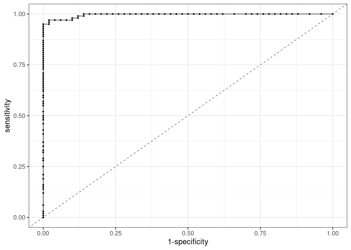
The AUC is much closer to one now:
iris_rf |>
  roc_auc(is_versicolor, .pred_versicolor)
## # A tibble: 1 × 3
## .metric .estimator .estimate
## <chr> <chr> <dbl>
## 1 roc_auc binary 0.996A Bad ROC Curve
Let’s see the behaviour of a very bad classifier. We define the probability of each observation of being versicolor as a random value between zero and one:
iris_awful <- iris |>
  mutate(.pred_versicolor = runif(150, 0, 1))
If we define the ROC curve for this classifier, we observe that it lays around the diagonal:
roc_iris_awful <- iris_awful |>
  roc_curve(truth = is_versicolor, estimate = .pred_versicolor) |>
  mutate(x_roc = 1-sensitivity, y_roc=specificity)

sens_spec_awful <- roc_iris_awful |>
  filter(.threshold > 0.48, .threshold < .52)


roc_iris_awful |>
  ggplot(aes(x_roc, y_roc)) +
  geom_point(size=0.5) +
  geom_point(data=sens_spec_awful, aes(x_roc, y_roc), size=3, color="red") +
  geom_line(size=0.3, color = "#808080") +
  geom_abline(slope=1, intercept = 0, linetype = "dashed", size=0.2) +
  theme_bw() +
  labs(x="1-specificity", y="sensitivity")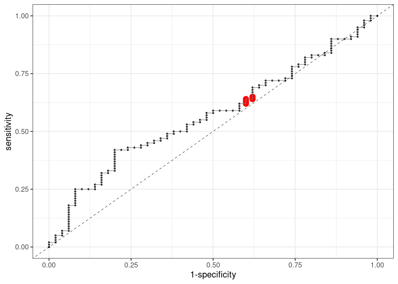
… and that the AUC is close to is lower bound 0.5:
iris_awful |>
  roc_auc(is_versicolor, .pred_versicolor)
## # A tibble: 1 × 3
## .metric .estimator .estimate
## <chr> <chr> <dbl>
## 1 roc_auc binary 0.571Assessing Model Performance with ROC and AUC
With a bad classifier, if we want to increase sensitivity (the ability to predict the positive class) we need to reduce specificity (the ability to predict the negative class). That’s why the ROC curve of a bad classifier lies close to the diagonal. A good classifier will yield good values of sensitivity and sensibility at once. This means that its ROC curve will be closer to the upper left corner, and the area under the curve (AUC) will be closer to one. ROC and AUC measure of how classifier is able to separate positive and negative cases. In fact, it was developed by radar engineers in World War II to measure the ability of a radar to detect objects depending on the threshold value of detection.
References
- Understanding AUC/ROC curve, by Sarang Narkhede https://towardsdatascience.com/understanding-auc-roc-curve-68b2303cc9c5
Session Info
## R version 4.2.2 Patched (2022-11-10 r83330)
## Platform: x86_64-pc-linux-gnu (64-bit)
## Running under: Linux Mint 21.1
##
## Matrix products: default
## BLAS:   /usr/lib/x86_64-linux-gnu/blas/libblas.so.3.10.0
## LAPACK: /usr/lib/x86_64-linux-gnu/lapack/liblapack.so.3.10.0
##
## locale:
##  [1] LC_CTYPE=es_ES.UTF-8       LC_NUMERIC=C
##  [3] LC_TIME=es_ES.UTF-8        LC_COLLATE=es_ES.UTF-8
##  [5] LC_MONETARY=es_ES.UTF-8    LC_MESSAGES=es_ES.UTF-8
##  [7] LC_PAPER=es_ES.UTF-8       LC_NAME=C
##  [9] LC_ADDRESS=C               LC_TELEPHONE=C
## [11] LC_MEASUREMENT=es_ES.UTF-8 LC_IDENTIFICATION=C
##
## attached base packages:
## [1] stats     graphics  grDevices utils     datasets  methods   base
##
## other attached packages:
##  [1] yardstick_1.1.0    workflowsets_1.0.0 workflows_1.1.2    tune_1.0.1
##  [5] tidyr_1.3.0        tibble_3.1.8       rsample_1.1.1      recipes_1.0.4
##  [9] purrr_1.0.1        parsnip_1.0.3      modeldata_1.1.0    infer_1.0.4
## [13] ggplot2_3.4.0      dplyr_1.0.10       dials_1.1.0        scales_1.2.1
## [17] broom_1.0.3        tidymodels_1.0.0
##
## loaded via a namespace (and not attached):
##  [1] sass_0.4.5          foreach_1.5.2       jsonlite_1.8.4
##  [4] splines_4.2.2       prodlim_2019.11.13  bslib_0.4.2
##  [7] assertthat_0.2.1    highr_0.10          GPfit_1.0-8
## [10] yaml_2.3.7          globals_0.16.2      ipred_0.9-13
## [13] pillar_1.8.1        backports_1.4.1     lattice_0.20-45
## [16] glue_1.6.2          digest_0.6.31       hardhat_1.2.0
## [19] colorspace_2.1-0    htmltools_0.5.4     Matrix_1.5-1
## [22] timeDate_4022.108   pkgconfig_2.0.3     lhs_1.1.6
## [25] DiceDesign_1.9      listenv_0.9.0       bookdown_0.32
## [28] ranger_0.14.1       gower_1.0.1         lava_1.7.1
## [31] timechange_0.2.0    farver_2.1.1        generics_0.1.3
## [34] ellipsis_0.3.2      cachem_1.0.6        withr_2.5.0
## [37] furrr_0.3.1         nnet_7.3-18         cli_3.6.0
## [40] survival_3.5-3      magrittr_2.0.3      evaluate_0.20
## [43] future_1.31.0       fansi_1.0.4         parallelly_1.34.0
## [46] MASS_7.3-58.2       class_7.3-21        blogdown_1.16
## [49] tools_4.2.2         lifecycle_1.0.3     munsell_0.5.0
## [52] compiler_4.2.2      jquerylib_0.1.4     rlang_1.0.6
## [55] grid_4.2.2          iterators_1.0.14    rstudioapi_0.14
## [58] labeling_0.4.2      rmarkdown_2.20      gtable_0.3.1
## [61] codetools_0.2-19    DBI_1.1.3           R6_2.5.1
## [64] lubridate_1.9.1     knitr_1.42          fastmap_1.1.0
## [67] future.apply_1.10.0 utf8_1.2.2          parallel_4.2.2
## [70] Rcpp_1.0.10         vctrs_0.5.2         rpart_4.1.19
## [73] tidyselect_1.2.0    xfun_0.36
Updated at 2023-03-20 10:41:17.