tidymodels is a collection of packages for modelling and machine learning in R, drawing on the tools and approach of the tidyverse. It is replacing caret as the main choice to work in supervised learning models.
The best way to start with tidymodels is with a small example. I have found this example of multiclass classification with the iris dataset very helpful. Here I will present a similar workflow, but with a binary classification problem. Loading tidymodels only, we’ll have all the packages we need:
library(tidymodels)Our job is to build a model predicting if an iris flower is of the species versicolor. This is a binary classification problem. It has some difficulty, as versicolor are close to virginica:
ggplot(iris, aes(Sepal.Length, Sepal.Width, color = Species)) +
  geom_point(size=1.5) +
  theme_bw()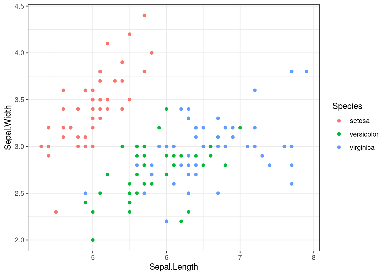
Let’s define the target variable. When using tidymodels in binary classification problems, the target variable:
- must be a factor,
- with its first level corresponding to the positive class.
iris <- iris |>
  mutate(is_versicolor = ifelse(Species == "versicolor", "versicolor", "not_versicolor")) |>
  mutate(is_versicolor = factor(is_versicolor, levels = c("versicolor", "not_versicolor")))
In binary classification problems, the class associated with the presence of a property is labelled positive. Here the positive class is that the flower is versicolor, that is is_versicolor==versicolor. The other class is labelled negative. Here that means that the flower is not versicolor is_versicolor==not_versicolor.
Data Preprocessing with recipes
Data pre-processing in tidymodels is performed with the recipes package. A recipe has the following structure:
iris_recipe <- iris |>
  recipe(is_versicolor ~.) |>
  step_rm(Species) |>
  step_corr(all_predictors()) |>
  step_center(all_predictors(), -all_outcomes()) |>
  step_scale(all_predictors(), -all_outcomes())
The components of this recipe are:
- The data to apply the recipe, in this case the whole
iris. - A
recipeinstruction defining the model: here we state thatis_versicoloris the target variable, and the remaining variables the features. - Some steps to transform data. Here we remove
Specieswithstep_rm, look for correlated predictors withstep_corr, center (substract the mean) and scale (divide by standard deviation) the predictors withstep_scale.
To see what the recipe has done we can just estimate doing:
iris_recipe |>
  prep()
## Recipe
##
## Inputs:
##
## role #variables
## outcome 1
## predictor 5
##
## Training data contained 150 data points and no missing data.
##
## Operations:
##
## Variables removed Species [trained]
## Correlation filter on Petal.Length [trained]
## Centering for Sepal.Length, Sepal.Width, Petal.Width [trained]
## Scaling for Sepal.Length, Sepal.Width, Petal.Width [trained]We see that the recipe has removed Petal.Length because it was highly correlated with other variables. The next steps of the recipe have not been applied to that variable, so the order in which to apply the steps is relevant.
Defining the Model with parsnip
The models in tidymodels are stored in parsnip, the successor of caret (whence its name). Here we define a random forest model with some parameters and specify the engine we are using. The engine in the parsnip context is the source of the code to run the model. It can be a package, a R base function, stan or spark, among others. Here we are using the random forest implemented in the ranger package.
rf <- rand_forest(mode = "classification", trees = 100) |>
  set_engine("ranger")
Defining a workflow
Once we have a model and a recipe, we can put it all together with a workflow:
iris_rf_wf <- workflow() |>
  add_recipe(iris_recipe) |>
  add_model(rf)
The workflow iris_rf_wf applies the preprocess recipe iris_recipe, and then builds the model rf with data applied to that recipe.
Obtaining Predictions
When we fitthe workflow to iris, we obtain model hyperparameters using the iris dataset. Then, we can predict the class of each observation from the same data. As the outcome is set in a tibble format, we can use bind_cols to attach the prediction to the original data set.
set.seed(3131)
iris_pred <- iris_rf_wf |>
  fit(iris) |>
  predict(iris) |>
  bind_cols(iris)
Let’s examine the results:
iris_pred |>
  glimpse()
## Rows: 150
## Columns: 7
## $ .pred_class <fct> not_versicolor, not_versicolor, not_versicolor, not_vers…
## $ Sepal.Length <dbl> 5.1, 4.9, 4.7, 4.6, 5.0, 5.4, 4.6, 5.0, 4.4, 4.9, 5.4, 4…
## $ Sepal.Width <dbl> 3.5, 3.0, 3.2, 3.1, 3.6, 3.9, 3.4, 3.4, 2.9, 3.1, 3.7, 3…
## $ Petal.Length <dbl> 1.4, 1.4, 1.3, 1.5, 1.4, 1.7, 1.4, 1.5, 1.4, 1.5, 1.5, 1…
## $ Petal.Width <dbl> 0.2, 0.2, 0.2, 0.2, 0.2, 0.4, 0.3, 0.2, 0.2, 0.1, 0.2, 0…
## $ Species <fct> setosa, setosa, setosa, setosa, setosa, setosa, setosa, …
## $ is_versicolor <fct> not_versicolor, not_versicolor, not_versicolor, not_vers…We have the predicted outcome in the .pred_class variable. Note that the variable omitted in the recipe has not been removed from the dataset.
Evaluating model performance
We can examine how well has performed the model with the confusion matrix:
iris_pred |>
  conf_mat(truth = is_versicolor, estimate = .pred_class)
## Truth
## Prediction versicolor not_versicolor
## versicolor 49 3
## not_versicolor 1 97Let’s define a metric_set including the following parameters:
- accuracy: the fraction of observations correctly classified,
- sensibility: the fraction of positive observations correctly classified,
- specificity: the fraction of negative observations correctly classified.
The obtained values are:
class_metrics <- metric_set(accuracy, sens, spec)and estimate the values:
iris_pred |>
 class_metrics(truth = is_versicolor, estimate = .pred_class)
## # A tibble: 3 × 3
## .metric .estimator .estimate
## <chr> <chr> <dbl>
## 1 accuracy binary 0.973
## 2 sens binary 0.98
## 3 spec binary 0.97Here we see that
- accuracy is (49+97)/(49+97+3+1) = 0.073,
- sensibility is equal to 49/(1+49) = 0.980,
- specificity is equal to 97/(97+3) = 0.970.
More Features of tidymodels
This is a very basic workflow of model training with tidymodels. There are many more features available, among others:
- train models of regression or numerical prediction,
- define train and test sets, and test models with cross validation,
- tune hyperparameter models,
- use subsampling with unbalanced datasets,
- use more performance metrics to build the model.
References
recipesfunction reference: https://recipes.tidymodels.org/reference/index.html- list of available models in
parsnip: https://www.tidymodels.org/find/parsnip/
Session Info
## R version 4.2.2 Patched (2022-11-10 r83330)
## Platform: x86_64-pc-linux-gnu (64-bit)
## Running under: Linux Mint 21.1
##
## Matrix products: default
## BLAS:   /usr/lib/x86_64-linux-gnu/blas/libblas.so.3.10.0
## LAPACK: /usr/lib/x86_64-linux-gnu/lapack/liblapack.so.3.10.0
##
## locale:
##  [1] LC_CTYPE=es_ES.UTF-8       LC_NUMERIC=C
##  [3] LC_TIME=es_ES.UTF-8        LC_COLLATE=es_ES.UTF-8
##  [5] LC_MONETARY=es_ES.UTF-8    LC_MESSAGES=es_ES.UTF-8
##  [7] LC_PAPER=es_ES.UTF-8       LC_NAME=C
##  [9] LC_ADDRESS=C               LC_TELEPHONE=C
## [11] LC_MEASUREMENT=es_ES.UTF-8 LC_IDENTIFICATION=C
##
## attached base packages:
## [1] stats     graphics  grDevices utils     datasets  methods   base
##
## other attached packages:
##  [1] yardstick_1.1.0    workflowsets_1.0.0 workflows_1.1.2    tune_1.0.1
##  [5] tidyr_1.3.0        tibble_3.1.8       rsample_1.1.1      recipes_1.0.4
##  [9] purrr_1.0.1        parsnip_1.0.3      modeldata_1.1.0    infer_1.0.4
## [13] ggplot2_3.4.0      dplyr_1.0.10       dials_1.1.0        scales_1.2.1
## [17] broom_1.0.3        tidymodels_1.0.0
##
## loaded via a namespace (and not attached):
##  [1] sass_0.4.5          foreach_1.5.2       jsonlite_1.8.4
##  [4] splines_4.2.2       prodlim_2019.11.13  bslib_0.4.2
##  [7] assertthat_0.2.1    highr_0.10          GPfit_1.0-8
## [10] yaml_2.3.7          globals_0.16.2      ipred_0.9-13
## [13] pillar_1.8.1        backports_1.4.1     lattice_0.20-45
## [16] glue_1.6.2          digest_0.6.31       hardhat_1.2.0
## [19] colorspace_2.1-0    htmltools_0.5.4     Matrix_1.5-1
## [22] timeDate_4022.108   pkgconfig_2.0.3     lhs_1.1.6
## [25] DiceDesign_1.9      listenv_0.9.0       bookdown_0.32
## [28] ranger_0.14.1       gower_1.0.1         lava_1.7.1
## [31] timechange_0.2.0    farver_2.1.1        generics_0.1.3
## [34] ellipsis_0.3.2      cachem_1.0.6        withr_2.5.0
## [37] furrr_0.3.1         nnet_7.3-18         cli_3.6.0
## [40] survival_3.5-3      magrittr_2.0.3      evaluate_0.20
## [43] future_1.31.0       fansi_1.0.4         parallelly_1.34.0
## [46] MASS_7.3-58.2       class_7.3-21        blogdown_1.16
## [49] tools_4.2.2         lifecycle_1.0.3     munsell_0.5.0
## [52] compiler_4.2.2      jquerylib_0.1.4     rlang_1.0.6
## [55] grid_4.2.2          iterators_1.0.14    rstudioapi_0.14
## [58] labeling_0.4.2      rmarkdown_2.20      gtable_0.3.1
## [61] codetools_0.2-19    DBI_1.1.3           R6_2.5.1
## [64] lubridate_1.9.1     knitr_1.42          fastmap_1.1.0
## [67] future.apply_1.10.0 utf8_1.2.2          parallel_4.2.2
## [70] Rcpp_1.0.10         vctrs_0.5.2         rpart_4.1.19
## [73] tidyselect_1.2.0    xfun_0.36
Updated at 2023-03-20 10:29:54