This post is the making of the previous post about measures of inequality. I will present how I have:
- defined the three income distributions.
- obtained the mean to median ratio for each distribution.
- defined an efficient function to calculate the Gini index.
- obtained the Lorenz curve plots.
I have used the tidyverse to do all the jobs and kableExtra to present tables.
library(tidyverse)
library(kableExtra)
Defining Income Distributions
I start defining an income table with three distributions progressively more unequal. r1 is a sample of a normal distribution, and r2 and r3 are samples of right skewed distributions obtaining powering 10 with the values of a normal distribution. The standard deviation of r3 is higher than r2, resulting in higher inequality.
set.seed(1111)
income <- tibble(id = 1:10000,
                 r1 = rnorm(10000, mean = 10000, sd = 100),
                 r2 = 10^rnorm(10000, mean = 4, sd = 0.2),
                 r3 = 10^rnorm(10000, mean = 4, sd = 0.5))
Let’s define an income_long tidy table with pivot_longer:
income_long <- income |>
  pivot_longer(-id)
income_long
## # A tibble: 30,000 × 3
## id name value
## <int> <chr> <dbl>
## 1 1 r1 9991.
## 2 1 r2 23019.
## 3 1 r3 15224.
## 4 2 r1 10132.
## 5 2 r2 9399.
## 6 2 r3 90306.
## 7 3 r1 10064.
## 8 3 r2 5118.
## 9 3 r3 92768.
## 10 4 r1 10117.
## # ℹ 29,990 more rowsPlotting the Histograms
The obvious choice to plot the three histograms is to use facet_grid:
income_long |>
  ggplot(aes(value)) +
  geom_histogram(bins = 40, fill = "#A0A0A0") +
      theme_minimal() +
      labs(x = NULL, y = NULL) +
      facet_grid(. ~ name)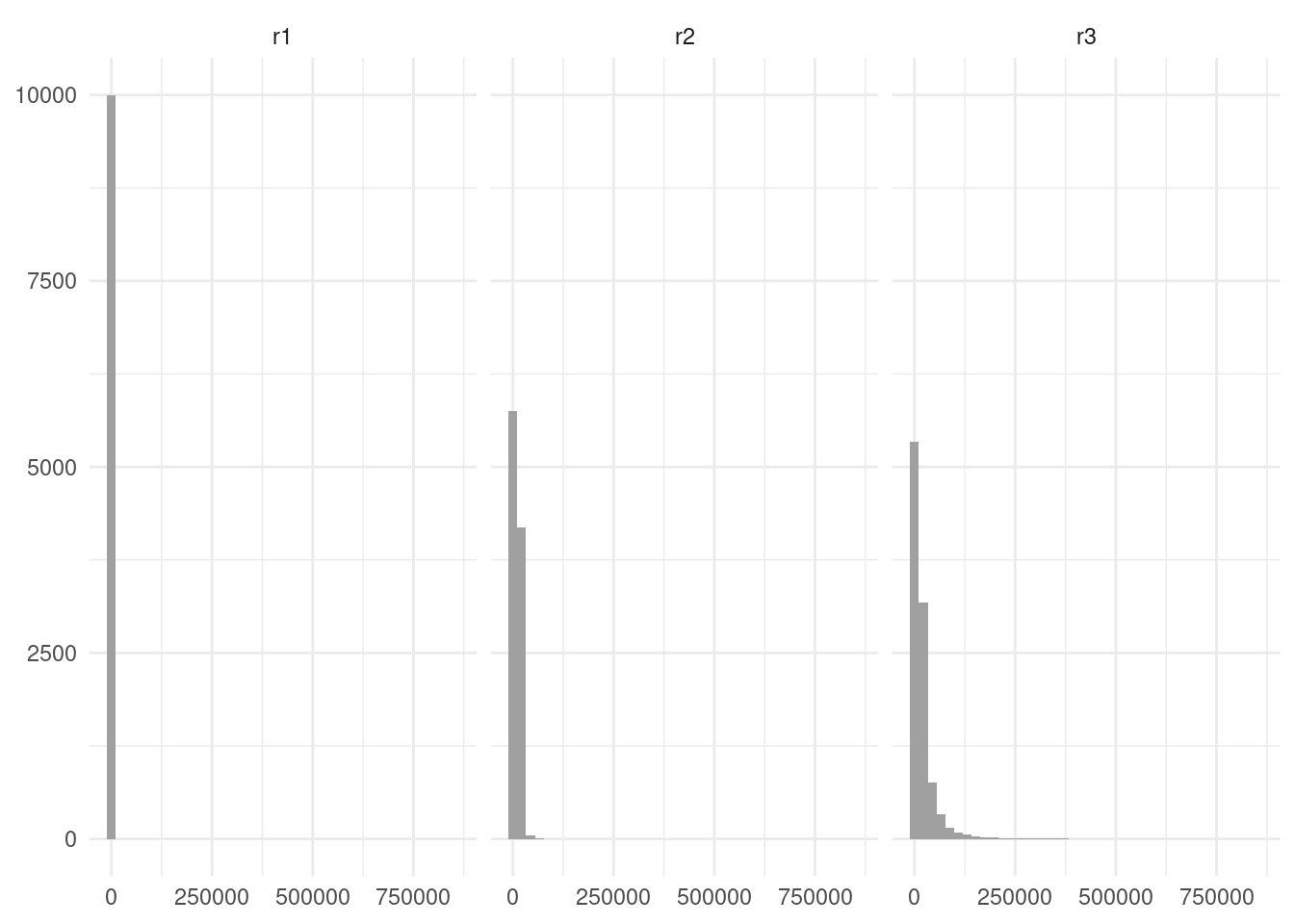
This first draft is not adequate as the ranges of values for each distribution are different. To remedy that, I have set scale = "free" argument in facet_grid. I have also changed the size and angle of x axis labels to avoid overlap.
income_long |>
  ggplot(aes(value)) +
  geom_histogram(bins = 40, fill = "#A0A0A0") +
      facet_grid(. ~ name, scales = "free") +
      theme_minimal() +
      theme(axis.title = element_blank(),
            axis.text.x = element_text(size = 10, angle = -45))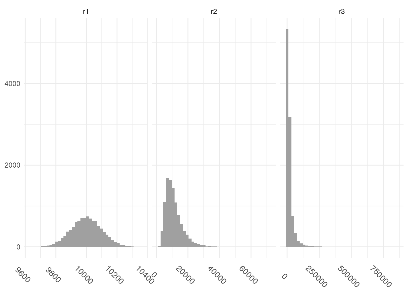
Mean to median Ratio
To obtain the mean to median ratio I need to summarise the mean and median, and then obtain the ratio with mutate. I can adjust the decimals to show with kbl:
income_long |>
  group_by(name) |>
  summarise(mean = mean(value), median = median(value)) |>
  mutate(ratio = mean/median) |>
  kbl(digits = 3) |>
kable_styling(full_width = FALSE)| name | mean | median | ratio |
|---|---|---|---|
| r1 | 9999.235 | 9999.347 | 1.000 |
| r2 | 11130.645 | 9979.472 | 1.115 |
| r3 | 19376.763 | 9911.144 | 1.955 |
Calculating the Gini Index
I need to define a function to implement this expression.
\[\frac{\displaystyle\sum_{i=1}^n \displaystyle\sum_{i=1}^n \vert x_i - x_j \vert}{2n^2\bar{x}} \]
The obvious path is the one defined in the gini2 function, looping twice across each element of the vector:
gini2 <- function(x){
  n <- length(x)
  sum <- 0

  for(i in 1:n)
    for(j in 1:n)
      sum <- sum + abs(x[i] - x[j])

  g <- sum / (2 * n^2 * mean(x))
  return(g)
}
But as R is a vectorial language, we can try an alternative to find all absolute differences without looping. I will define two square matrices: one with all rows equal and other with all columns equal. We can use the rep function to do this. We obtain the first matrix doing:
matrix(rep(1:10, each = 10), 10, 10)## [,1] [,2] [,3] [,4] [,5] [,6] [,7] [,8] [,9] [,10]
## [1,] 1 2 3 4 5 6 7 8 9 10
## [2,] 1 2 3 4 5 6 7 8 9 10
## [3,] 1 2 3 4 5 6 7 8 9 10
## [4,] 1 2 3 4 5 6 7 8 9 10
## [5,] 1 2 3 4 5 6 7 8 9 10
## [6,] 1 2 3 4 5 6 7 8 9 10
## [7,] 1 2 3 4 5 6 7 8 9 10
## [8,] 1 2 3 4 5 6 7 8 9 10
## [9,] 1 2 3 4 5 6 7 8 9 10
## [10,] 1 2 3 4 5 6 7 8 9 10And the second:
matrix(rep(1:10, times = 10), 10, 10)## [,1] [,2] [,3] [,4] [,5] [,6] [,7] [,8] [,9] [,10]
## [1,] 1 1 1 1 1 1 1 1 1 1
## [2,] 2 2 2 2 2 2 2 2 2 2
## [3,] 3 3 3 3 3 3 3 3 3 3
## [4,] 4 4 4 4 4 4 4 4 4 4
## [5,] 5 5 5 5 5 5 5 5 5 5
## [6,] 6 6 6 6 6 6 6 6 6 6
## [7,] 7 7 7 7 7 7 7 7 7 7
## [8,] 8 8 8 8 8 8 8 8 8 8
## [9,] 9 9 9 9 9 9 9 9 9 9
## [10,] 10 10 10 10 10 10 10 10 10 10So we obtain all differences doing:
abs(matrix(rep(1:10, each = 10), 10, 10) - matrix(rep(1:10, times = 10), 10, 10))## [,1] [,2] [,3] [,4] [,5] [,6] [,7] [,8] [,9] [,10]
## [1,] 0 1 2 3 4 5 6 7 8 9
## [2,] 1 0 1 2 3 4 5 6 7 8
## [3,] 2 1 0 1 2 3 4 5 6 7
## [4,] 3 2 1 0 1 2 3 4 5 6
## [5,] 4 3 2 1 0 1 2 3 4 5
## [6,] 5 4 3 2 1 0 1 2 3 4
## [7,] 6 5 4 3 2 1 0 1 2 3
## [8,] 7 6 5 4 3 2 1 0 1 2
## [9,] 8 7 6 5 4 3 2 1 0 1
## [10,] 9 8 7 6 5 4 3 2 1 0And the summmation:
sum(abs(matrix(rep(1:10, each = 10), 10, 10) - matrix(rep(1:10, times = 10), 10, 10)))## [1] 330We can obtain the same result substracting the vectors used to build the matrices:
sum(abs(rep(1:10, each = 10) - rep(1:10, times = 10)))## [1] 330So we can construct the function:
gini <- function(x){
  n <- length(x)
  g <- sum(abs(rep(x, times = n) - rep(x, each = n))) / (2 * n^2 * mean(x))
  return(g)
}
Let’s examine the performance of each function with rbenchmark:
rbenchmark::benchmark(replications = 10,
                      gini(income$r3),
                      gini2(income$r3),
                      columns=c('test', 'elapsed', 'relative', 'replications'),
                      order = 'elapsed')
## test elapsed relative replications
## 1 gini(income$r3) 24.455 1.00 10
## 2 gini2(income$r3) 109.318 4.47 10The non-looping function has better performance, so I will use gini to calculate gini indices of each distribution:
income |>
  summarise(across(r1:r3, gini)) |>
  kbl(digits = 3) |>
kable_styling(full_width = FALSE)| r1 | r2 | r3 |
|---|---|---|
| 0.006 | 0.258 | 0.587 |
Plotting Lorenz Curves
The last job is plotting Lorenz curves. To do so I need to calculate:
- the cumulative share of people from lower to higher income.
- he cumulative share of income earned by each share.
This can be achieved with dplyr functions:
arrangerows bynameandvalueof income in decreasing order.- obtain the cumulative fraction of individuals
frac_ind. - obtain the cumulative fraction of income using
cumsum.
income_long <-
  income_long |>
  arrange(name, value) |>
  group_by(name) |>
  mutate(frac_ind =1:n()/n(),
         frac_rent = cumsum(value)/sum(value), .groups = "drop")
Note that here I am combining group_by and mutate. As I am storing the result in income_long and I don’t need a grouping table, I am doing .groups = "drop" in mutate.
Now I am ready to plot the Lorenz curves. The area under the curve is filled with geom_polygon quite naturally in this case. For this plot, I have decided to use a pale yellow background to differentiate each curve visually adding a panel.background definition in theme.
income_long |>
  ggplot(aes(frac_ind, frac_rent)) +
  geom_line() +
  geom_polygon(fill = "#A0A0A0") +
  theme_minimal() +
  theme(panel.background = element_rect(fill = "#FFFFEE")) +
  labs(x=NULL, y=NULL) +
  facet_grid(. ~ name)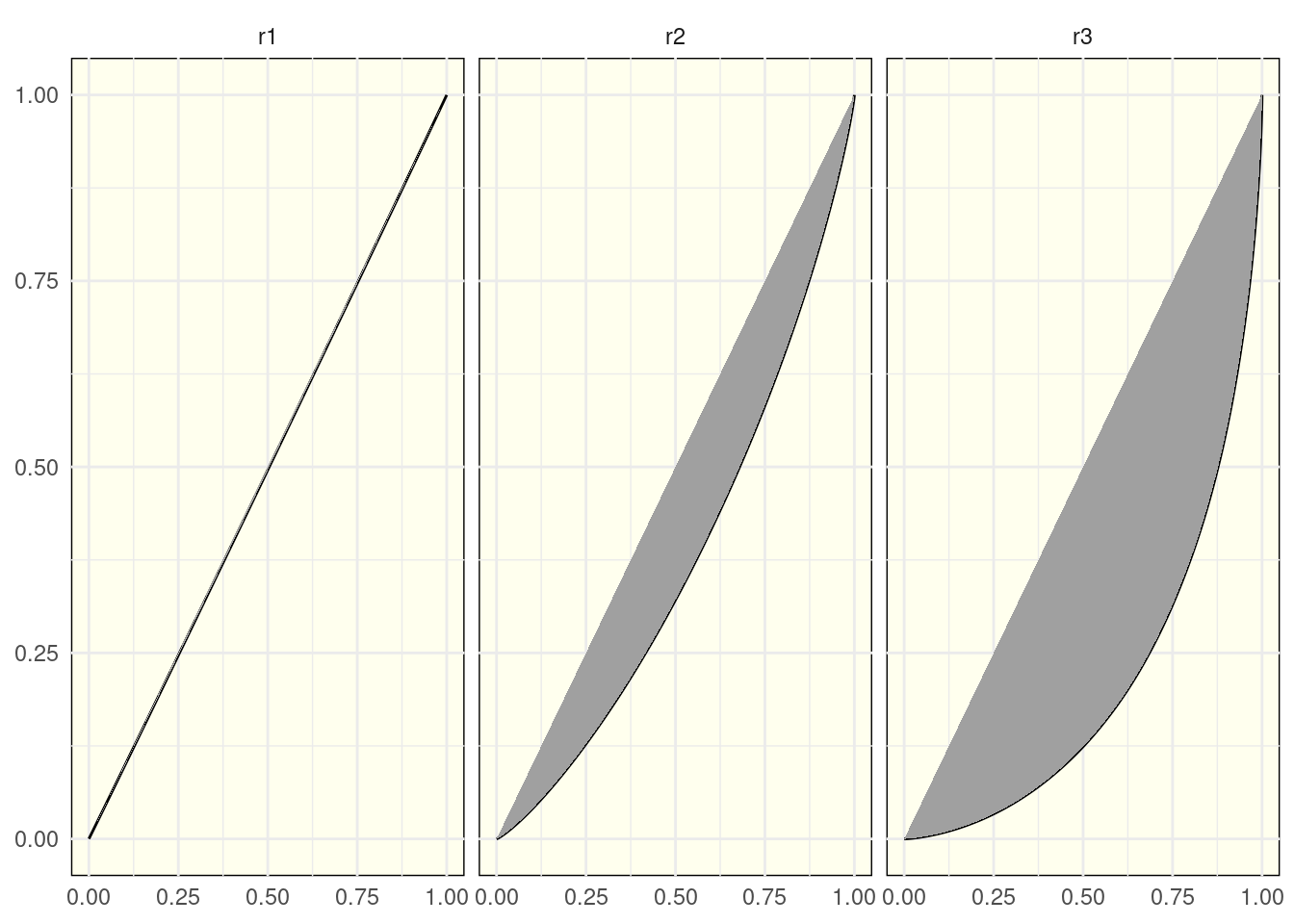
Session Info
## R version 4.3.0 (2023-04-21)
## Platform: x86_64-pc-linux-gnu (64-bit)
## Running under: Linux Mint 21.1
##
## Matrix products: default
## BLAS:   /usr/lib/x86_64-linux-gnu/blas/libblas.so.3.10.0
## LAPACK: /usr/lib/x86_64-linux-gnu/lapack/liblapack.so.3.10.0
##
## locale:
##  [1] LC_CTYPE=es_ES.UTF-8       LC_NUMERIC=C
##  [3] LC_TIME=es_ES.UTF-8        LC_COLLATE=es_ES.UTF-8
##  [5] LC_MONETARY=es_ES.UTF-8    LC_MESSAGES=es_ES.UTF-8
##  [7] LC_PAPER=es_ES.UTF-8       LC_NAME=C
##  [9] LC_ADDRESS=C               LC_TELEPHONE=C
## [11] LC_MEASUREMENT=es_ES.UTF-8 LC_IDENTIFICATION=C
##
## time zone: Europe/Madrid
## tzcode source: system (glibc)
##
## attached base packages:
## [1] stats     graphics  grDevices utils     datasets  methods   base
##
## other attached packages:
##  [1] kableExtra_1.3.4 lubridate_1.9.2  forcats_1.0.0    stringr_1.5.0
##  [5] dplyr_1.1.2      purrr_1.0.1      readr_2.1.4      tidyr_1.3.0
##  [9] tibble_3.2.1     ggplot2_3.4.2    tidyverse_2.0.0
##
## loaded via a namespace (and not attached):
##  [1] sass_0.4.5        utf8_1.2.3        generics_0.1.3    xml2_1.3.3
##  [5] blogdown_1.16     stringi_1.7.12    hms_1.1.3         digest_0.6.31
##  [9] magrittr_2.0.3    evaluate_0.20     grid_4.3.0        timechange_0.2.0
## [13] bookdown_0.33     fastmap_1.1.1     jsonlite_1.8.4    httr_1.4.5
## [17] rvest_1.0.3       fansi_1.0.4       viridisLite_0.4.1 scales_1.2.1
## [21] jquerylib_0.1.4   cli_3.6.1         rlang_1.1.0       munsell_0.5.0
## [25] withr_2.5.0       cachem_1.0.7      yaml_2.3.7        tools_4.3.0
## [29] rbenchmark_1.0.0  tzdb_0.3.0        colorspace_2.1-0  webshot_0.5.4
## [33] vctrs_0.6.2       R6_2.5.1          lifecycle_1.0.3   pkgconfig_2.0.3
## [37] pillar_1.9.0      bslib_0.4.2       gtable_0.3.3      glue_1.6.2
## [41] systemfonts_1.0.4 highr_0.10        xfun_0.39         tidyselect_1.2.0
## [45] rstudioapi_0.14   knitr_1.42        farver_2.1.1      htmltools_0.5.5
## [49] labeling_0.4.2    svglite_2.1.1     rmarkdown_2.21    compiler_4.3.0