One of the key elements of predicting modelling workflow is feature selection. It is frequent that original data must be transformed in some way, as they may impact on model performance without additional computational complexity. A frequent data transformation in predictive modelling is principal component analysis (PCA). PCA returns a set of latent variables or components that capture a significant proportion of dataset variability. As components are uncorrelated, each of them is a distinct source of variability and solve multicollinearity issues.
To illustrate PCA transformation in the tidymodels framework, I will train a logistic regression model on the Sonar dataset fromt the mlbench package.
library(tidymodels)
library(mlbench)
The task of the Sonar dataset is to train a network to discriminate between sonar signals bounced off a metal cylinder M and those bounced off a roughly cylindrical rock R. The object to which correspond each set of signals is stored in the Class variable. Each pattern is a set of 60 numbers in the range 0.0 to 1.0. Each number represents the energy within a particular frequency band, integrated over a certain period of time. The signals are encoded in the V01 to V60 variables.
data("Sonar")When representing the proportion of each case, we observe that the number of positive (M case) and negative (R case) observations is balanced. As the first level corresponds with the positive case, no relevelling of the target variable is required.
Sonar |>
  ggplot(aes(Class)) +
  geom_bar(aes(y = after_stat(count/sum(count)))) +
  scale_y_continuous(name = NULL, labels = scales::percent) +
  ggtitle(label = "Proportion of positive and negative cases") +
  theme_minimal(base_size = 12)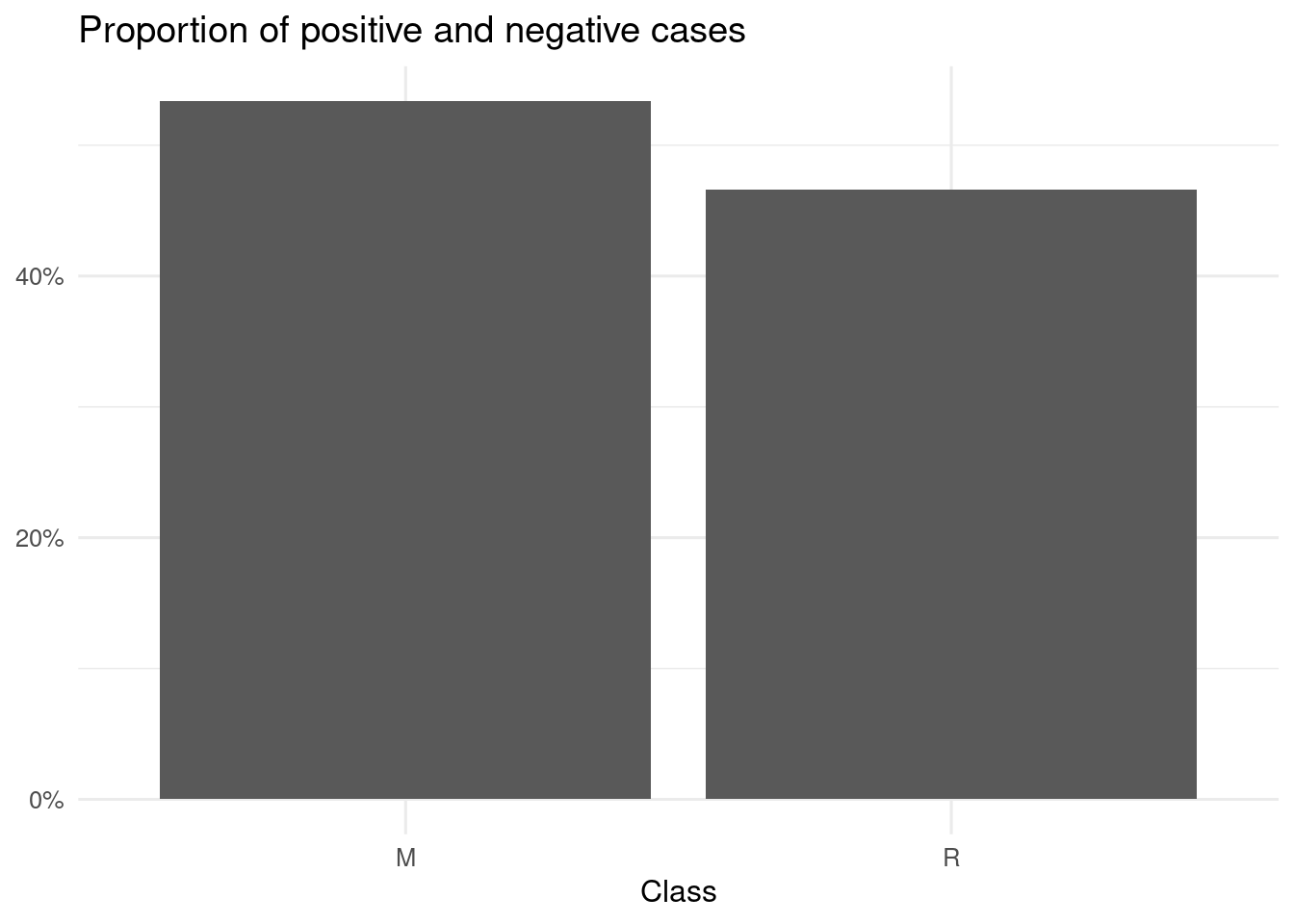
A Straight Logistic Regression
Let’s set the elements for a predictive modelling framework. First, we split the dataset into train an test.
set.seed(1111)
sonar_split <- initial_split(Sonar, prop = 0.8, strata = "Class")
Then, we define the set of metrics mset and the folds for cross validation folds.
mset <- metric_set(accuracy, sens, spec)
set.seed(1111)
folds <- vfold_cv(training(sonar_split), v = 5, repeats = 4, strata = "Class")
The preprocessing sonar_plain recipe includes only scaling and centering of predictors.
sonar_plain <- training(sonar_split) |>
  recipe(Class ~ .) |>
  step_center(all_numeric_predictors()) |>
  step_scale(all_numeric_predictors())
The model to apply is quite simple, a logistic regression lr with the R base function glm().
lr <- logistic_reg(mode = "classification",
                    engine = "glm")
Let’s examine the performance of the model with cross validation, and store the results in the lr_plain_cv data frame.
lr_plain_cv <- fit_resamples(object = lr,
                             preprocessor = sonar_plain,
                             resamples = folds,
                             metrics = mset) |>
  collect_metrics()
## → A | warning: glm.fit: algorithm did not converge, glm.fit: fitted probabilities numerically 0 or 1 occurred## There were issues with some computations A: x1## There were issues with some computations A: x6## There were issues with some computations A: x20## lr_plain_cv## # A tibble: 3 × 6
## .metric .estimator mean n std_err .config
## <chr> <chr> <dbl> <int> <dbl> <chr>
## 1 accuracy binary 0.708 20 0.0180 Preprocessor1_Model1
## 2 sens binary 0.705 20 0.0246 Preprocessor1_Model1
## 3 spec binary 0.712 20 0.0254 Preprocessor1_Model1Here we observe that the model has computational issues, as the algorithm does not converge and finds probabilities numerically 0 or 1 for some folds.
Features with Principal Component Analysis (PCA)
Let’s try the PCA approach, where we train the model with a set of latent variables uncorrelated with each other. We perform this transformation in tidymodels with step_pca(). It has two alternative tuning parameters:
num_compto specify the number of latent variables.thresholdto specify the fraction of total variance to be covered by the components.
Here I have chosen to pick as the number of components that accounts for an 80% of variance.
sonar_pca <- training(sonar_split) |>
  recipe(Class ~ .) |>
  step_center(all_numeric_predictors()) |>
  step_scale(all_numeric_predictors()) |>
  step_pca(all_numeric_predictors(),
           threshold = 0.8, prefix = "pc_")
If we examine the dataset obtained by the recipe, we observe that now we have 13 explanatory variables instead of 60.
sonar_pca |>
  prep() |>
  juice()
## # A tibble: 165 × 14
## Class pc_01 pc_02 pc_03 pc_04 pc_05 pc_06 pc_07 pc_08 pc_09 pc_10
## <fct> <dbl> <dbl> <dbl> <dbl> <dbl> <dbl> <dbl> <dbl> <dbl> <dbl>
## 1 M -6.16 1.62 3.05 1.90 -1.30 2.60 -1.69 1.91 4.37 -0.890
## 2 M -4.89 7.04 1.06 5.07 -6.82 3.26 -1.38 6.27 -3.17 3.11
## 3 M -2.25 1.81 2.26 2.11 -2.73 -1.30 0.302 -0.689 2.29 -2.75
## 4 M 0.147 8.17 2.89 0.812 -3.45 -2.50 0.0674 1.22 -1.51 -2.07
## 5 M -0.550 6.76 3.23 1.75 -1.63 -2.56 -0.127 1.09 -1.96 -1.02
## 6 M 2.54 4.95 4.05 -0.808 1.85 -3.19 -0.508 -0.433 -1.14 -2.72
## 7 M 0.0944 1.38 2.64 2.10 2.62 0.292 0.284 0.722 -0.465 0.193
## 8 M 0.548 2.42 2.29 1.19 2.59 1.31 -1.56 1.18 -0.302 -0.108
## 9 M 1.51 2.59 3.03 1.18 2.72 1.38 0.138 0.412 -0.342 -1.27
## 10 M 1.12 0.865 -0.320 3.55 2.77 1.63 0.658 -0.653 0.538 1.48
## # ℹ 155 more rows
## # ℹ 3 more variables: pc_11 <dbl>, pc_12 <dbl>, pc_13 <dbl>Predicting with PCA Features
Let’s test with cross validation the model including the PCA preprocessing.
lr_pca_cv <- fit_resamples(object = lr,
                           preprocessor = sonar_pca,
                           resamples = folds,
                           metrics = mset) |>
  collect_metrics()

lr_pca_cv
## # A tibble: 3 × 6
## .metric .estimator mean n std_err .config
## <chr> <chr> <dbl> <int> <dbl> <chr>
## 1 accuracy binary 0.769 20 0.0126 Preprocessor1_Model1
## 2 sens binary 0.789 20 0.0218 Preprocessor1_Model1
## 3 spec binary 0.747 20 0.0206 Preprocessor1_Model1Contrarily to the previous model, now we have no warnings about model convergence.
Comparing Models
Let’s compare the performance of each model. First I keep the columns that we need for each of the results of the cross validation, and bind both tables together.
lr_plain_cv <- lr_plain_cv |>
  mutate(model = "no PCA") |>
  select(.metric, mean, std_err, model)

lr_pca_cv <- lr_pca_cv |>
  mutate(model = "PCA") |>
  select(.metric, mean, std_err, model)

lr_table <- bind_rows(lr_plain_cv, lr_pca_cv)
Now we can represent each metric graphically for each model.
lr_table |>
  ggplot(aes(model, mean)) +
  geom_col(fill = "#C0C0C0", alpha = 0.5) +
  geom_errorbar(aes(model, ymin = mean - std_err/sqrt(20), ymax = mean + std_err/sqrt(20)), width = 0.3) +
  facet_grid(. ~ .metric) +
  theme_minimal(base_size = 12) +
  labs(title = "Logistic regression results", x = NULL, y = NULL)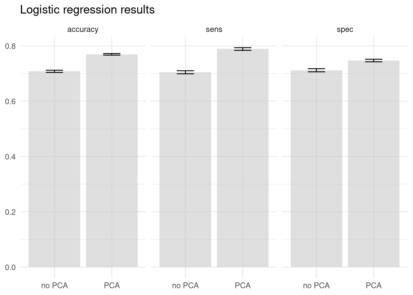
The use of PCA improves sensitivity and specificity, therefore improving accuracy.
Training the final model
We have chosen to train the logistic regression model with the PCA transformation. Let’s train the model with the whole training set, and assess performance on the test set.
lr_model <- workflow() |>
  add_recipe(sonar_pca) |>
  add_model(lr)

lr_trained_model <- lr_model |>
  fit(training(sonar_split))

lr_trained_model |>
  predict(testing(sonar_split)) |>
  bind_cols(testing(sonar_split) |> select(Class)) |>
  mset(truth = Class, estimate = .pred_class)
## # A tibble: 3 × 3
## .metric .estimator .estimate
## <chr> <chr> <dbl>
## 1 accuracy binary 0.791
## 2 sens binary 0.739
## 3 spec binary 0.85For the final model, results shows better performance on specificity spec and worse performance of sensitivity sens.
References
- Gorman, R. P., and Sejnowski, T. J. (1988). Analysis of Hidden Units in a Layered Network Trained to Classify Sonar Targets. Neural Networks, (1):75-89.
- A workflow for exploratory factor analysis in R. https://jmsallan.netlify.app/blog/a-workflow-for-exploratory-factor-analysis-in-r/.
- Why am I getting “algorithm did not converge” and “fitted prob numerically 0 or 1” warnings with glm? https://stackoverflow.com/questions/8596160/why-am-i-getting-algorithm-did-not-converge-and-fitted-prob-numerically-0-or
- PCA signal extraction. https://recipes.tidymodels.org/reference/step_pca.html
Session Info
## R version 4.4.2 (2024-10-31)
## Platform: x86_64-pc-linux-gnu
## Running under: Linux Mint 21.1
##
## Matrix products: default
## BLAS:   /usr/lib/x86_64-linux-gnu/blas/libblas.so.3.10.0
## LAPACK: /usr/lib/x86_64-linux-gnu/lapack/liblapack.so.3.10.0
##
## locale:
##  [1] LC_CTYPE=es_ES.UTF-8       LC_NUMERIC=C
##  [3] LC_TIME=es_ES.UTF-8        LC_COLLATE=es_ES.UTF-8
##  [5] LC_MONETARY=es_ES.UTF-8    LC_MESSAGES=es_ES.UTF-8
##  [7] LC_PAPER=es_ES.UTF-8       LC_NAME=C
##  [9] LC_ADDRESS=C               LC_TELEPHONE=C
## [11] LC_MEASUREMENT=es_ES.UTF-8 LC_IDENTIFICATION=C
##
## time zone: Europe/Madrid
## tzcode source: system (glibc)
##
## attached base packages:
## [1] stats     graphics  grDevices utils     datasets  methods   base
##
## other attached packages:
##  [1] mlbench_2.1-5      yardstick_1.3.1    workflowsets_1.1.0 workflows_1.1.4
##  [5] tune_1.2.1         tidyr_1.3.1        tibble_3.2.1       rsample_1.2.1
##  [9] recipes_1.0.10     purrr_1.0.2        parsnip_1.2.1      modeldata_1.3.0
## [13] infer_1.0.7        ggplot2_3.5.1      dplyr_1.1.4        dials_1.2.1
## [17] scales_1.3.0       broom_1.0.7        tidymodels_1.2.0
##
## loaded via a namespace (and not attached):
##  [1] tidyselect_1.2.1    timeDate_4032.109   farver_2.1.1
##  [4] fastmap_1.1.1       blogdown_1.19       digest_0.6.35
##  [7] rpart_4.1.24        timechange_0.3.0    lifecycle_1.0.4
## [10] ellipsis_0.3.2      survival_3.8-3      magrittr_2.0.3
## [13] compiler_4.4.2      rlang_1.1.5         sass_0.4.9
## [16] tools_4.4.2         utf8_1.2.4          yaml_2.3.8
## [19] data.table_1.15.4   knitr_1.46          labeling_0.4.3
## [22] DiceDesign_1.10     withr_3.0.0         nnet_7.3-20
## [25] grid_4.4.2          colorspace_2.1-0    future_1.33.2
## [28] globals_0.16.3      iterators_1.0.14    MASS_7.3-64
## [31] cli_3.6.2           rmarkdown_2.26      generics_0.1.3
## [34] rstudioapi_0.16.0   future.apply_1.11.2 cachem_1.0.8
## [37] splines_4.4.2       parallel_4.4.2      vctrs_0.6.5
## [40] hardhat_1.3.1       Matrix_1.7-2        jsonlite_1.8.9
## [43] bookdown_0.39       listenv_0.9.1       foreach_1.5.2
## [46] gower_1.0.1         jquerylib_0.1.4     glue_1.7.0
## [49] parallelly_1.37.1   codetools_0.2-19    lubridate_1.9.4
## [52] gtable_0.3.5        munsell_0.5.1       GPfit_1.0-8
## [55] pillar_1.10.1       furrr_0.3.1         htmltools_0.5.8.1
## [58] ipred_0.9-14        lava_1.8.0          R6_2.5.1
## [61] lhs_1.2.0           evaluate_0.23       lattice_0.22-5
## [64] highr_0.10          backports_1.4.1     bslib_0.7.0
## [67] class_7.3-23        Rcpp_1.0.12         prodlim_2023.08.28
## [70] xfun_0.43           pkgconfig_2.0.3