Exploring the Correlation mMatrix

The input of factor analysis is the correlation matrix, and for some indices the number of observations. We can explore correlations with the corrr package:

cor_tb <- correlate(hz)

corrr::rearrange groups highly correlated variables closer together, and corrr::rplot visualizes the result (I have used a custom color scale to highlight the results):

cor_tb |>
  rearrange() |>
  rplot(colors = c("red", "white", "blue"))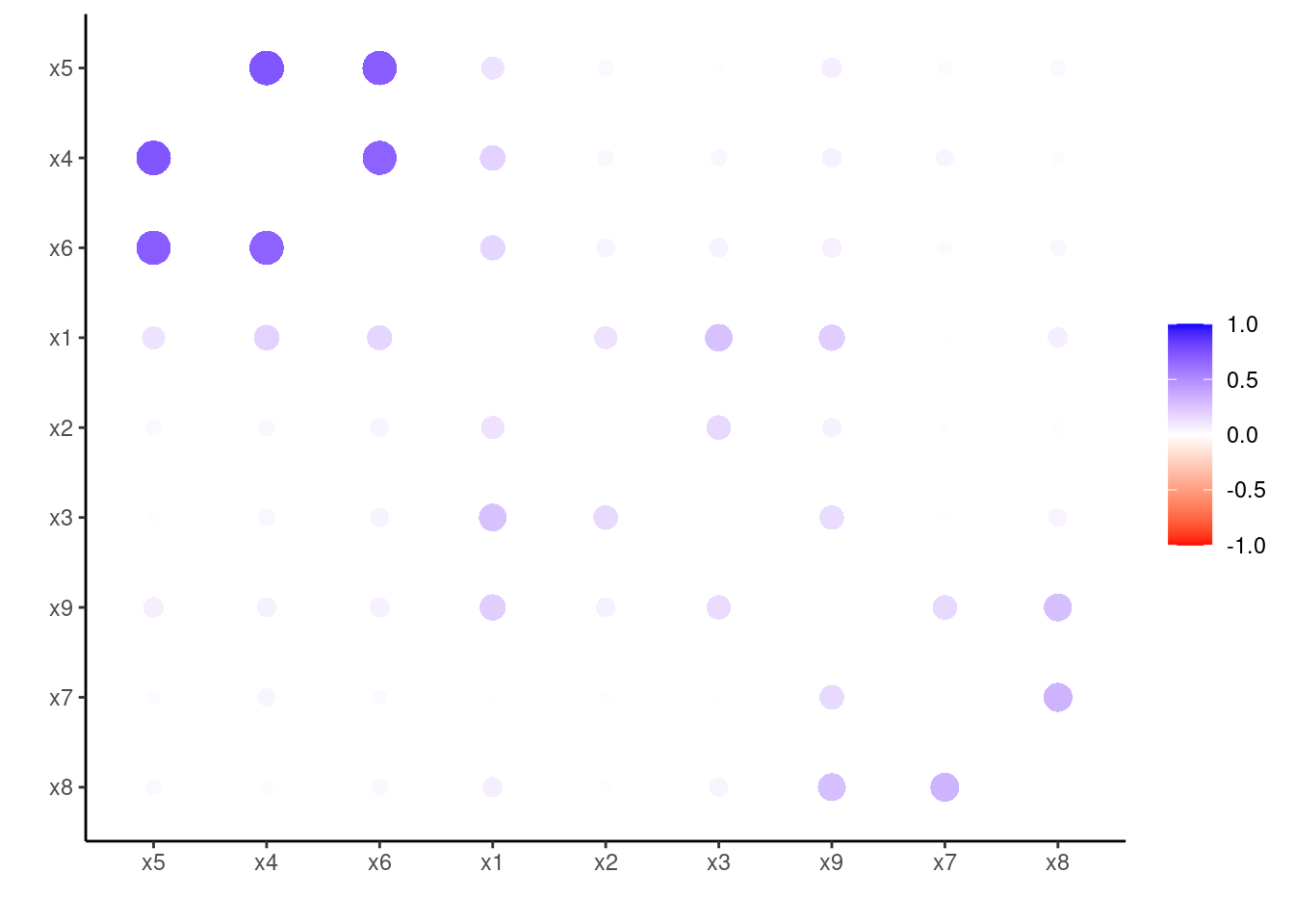

Looks like three groups emerge, around variables:

• x4 to x6 (first group).
• x1 to x3 (second group).
• x7 to x9 (third group).

Let’s start the factor analysis workflow. To do so, we need to obtain the correlations in matrix format with the R base cor function.

cor_mat <- cor(hz)

Preliminary tests

In preliminary analysis, we examine if the correlation matrix is suitable for factor analysis. We have two methods available:

• The Kaiser–Meyer–Olkin (KMO) test of sample adequacy. According to Kaiser (1974), values of KMO > 0.9 are marvelous, in the 0.80s, mertitourious, in the 0.70s, middling, in the 0.60s, mediocre, in the 0.50s, miserable, and less than 0.5, unacceptable. We can obtain that index with psych::KMO. It also provides a sample adequacy measure for each variable.
• The Bartlett’s test of sphericity. It is a testing of the hypothesis that the correlation matrix is an identity matrix. If this null hypothesis can be rejected, we can assume that variables are correlated and then perform factor analysis. We can do this testing with the psych::cortest.bartlett function.

The results of the KMO test are:

KMO(cor_mat)

## Kaiser-Meyer-Olkin factor adequacy
## Call: KMO(r = cor_mat)
## Overall MSA =  0.75
## MSA for each item = 
##   x1   x2   x3   x4   x5   x6   x7   x8   x9 
## 0.81 0.78 0.73 0.76 0.74 0.81 0.59 0.68 0.79

These eresults can be considered middling. The Bartlett’s test results are:

cortest.bartlett(R = cor_mat, n = 301)

## $chisq
## [1] 904.0971
## 
## $p.value
## [1] 1.912079e-166
## 
## $df
## [1] 36

Those results provide strong evidence that variables are correlated.

Number of Factors to Extract

A starting point to decide how many factors to extract is to examine the eigenvalues of correlation matrix.

eigen(cor_mat)$values

## [1] 3.2163442 1.6387132 1.3651593 0.6989185 0.5843475 0.4996872 0.4731021
## [8] 0.2860024 0.2377257

There are two criteria used to decide the number of factors to extract:

• Pick as many factors as eigenvalues greater than one.
• Examine the elbow point of the scree plot. In that plot we have the rank the factors in the x axis and the eigenvalues in the y axis.

Let’s do the scree plot to see the elbow point.

n <- dim(cor_mat)[1]
scree_tb <- tibble(x = 1:n, 
                   y = sort(eigen(cor_mat)$value, decreasing = TRUE))

scree_plot <- scree_tb |>
  ggplot(aes(x, y)) +
  geom_point() +
  geom_line() +
  theme_minimal() +
  scale_x_continuous(breaks = 1:n) +
  ggtitle("Scree plot")

scree_plot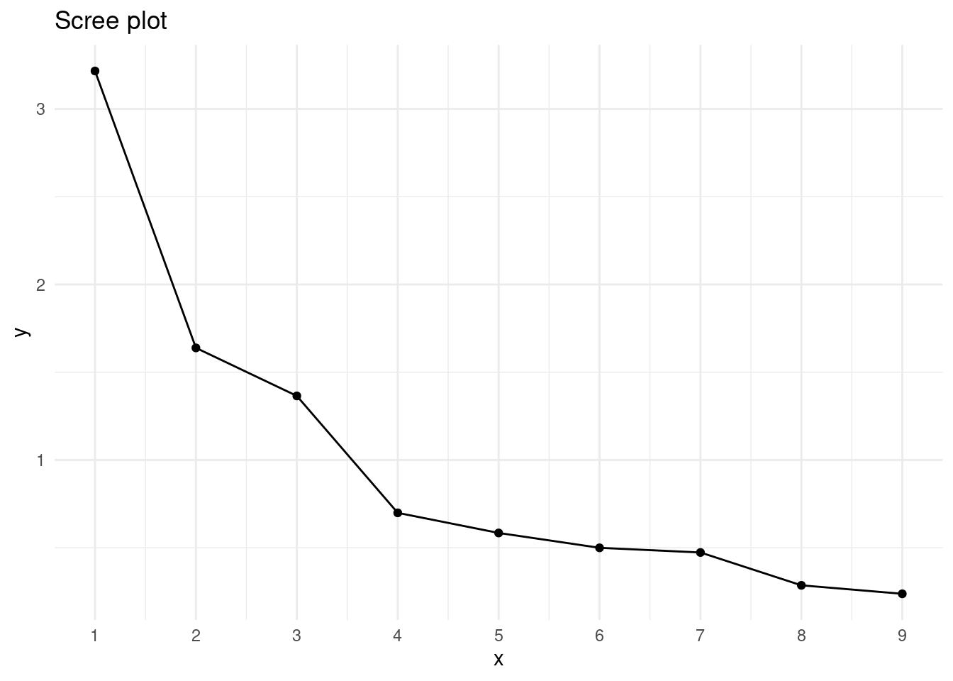

scree_plot +
  geom_vline(xintercept = 4, color = "red", linetype = "dashed") +
  annotate("text", 4.1, 2, label = "elbow point", color = "red", hjust = 0)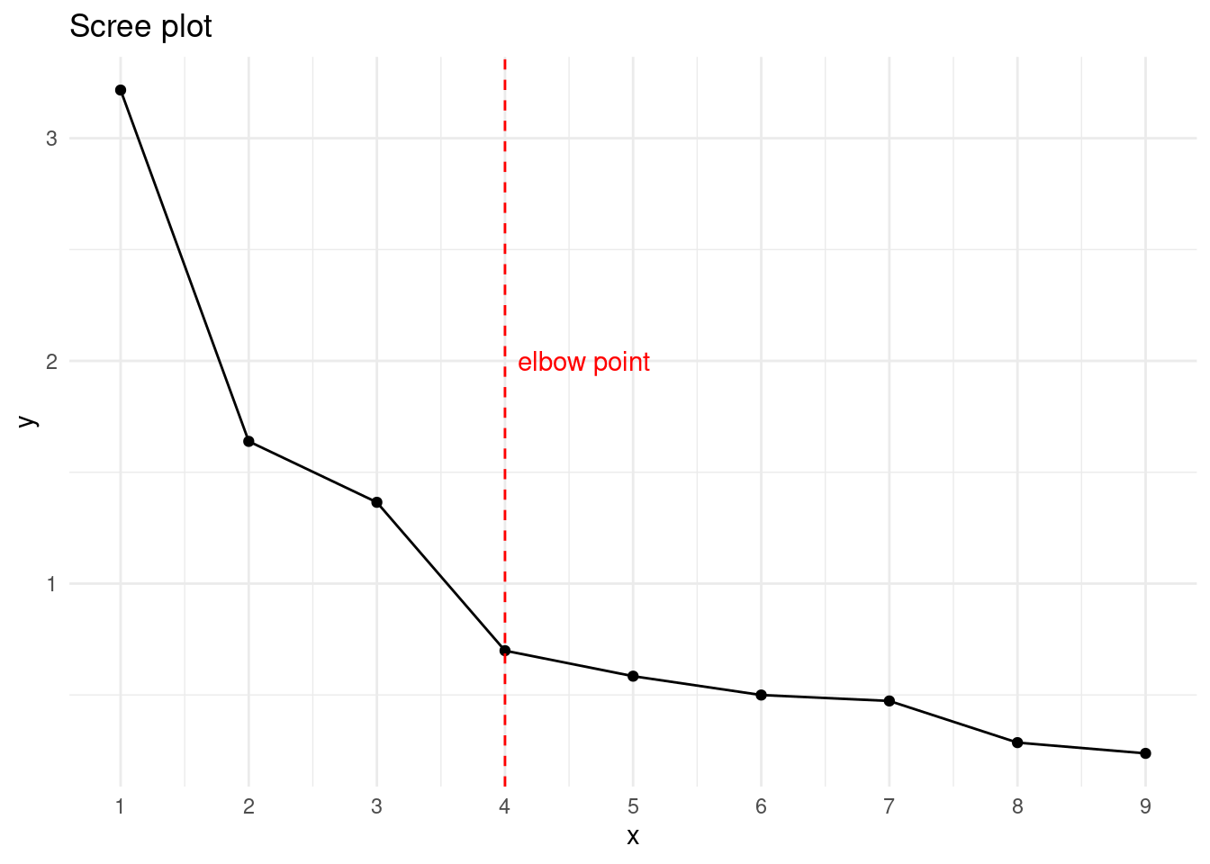

We observe that the elbow method occurs with four facgtor` and that we have three factors with eigenvalue greater than one. I have chosen to obtain a three-factor solution.

Factor Loadings and Rotations

Factor loedings \(f_{ij}\) are defined for each variable \(i\) and factor \(j\), and represent the correlation between both. A high value of \(f_{ij}\) means that a large amount of variability of variable \(i\) can be explained by factor \(j\).

Factor loadings of a model are unique up to a rotation. We prefer rotation methods that obtain factor loadings that allow relating one factor to each variable. Orthogonal rotations yield a set of uncorrelated factors. The most common orthogonal rotation methods are:

• Varimax maximizes variance of the squared loadings in each factor, so that each factor has only few variables with large loadings by the factor.
• Quartimax minimizes the number of factors needed to explain a variable.
• Equamax is a combination of varimax and quartimax.

Oblique rotations lead to a set of correlated factors. The most common oblique rotation methods are oblimin and promax.

In psych::fa, the type of rotation is passed with the rotate parameter.

For a factor analysis, we can split the variance of each variable in:

• Communality h2: the proportion of the variance explained by factors.
• Uniqueness u2: the proportion of the variance not explained by factors, thus unique for the variable.

Interpreting the Results

We can perform the factor analysis using the psych::fa function. This function allows several methods to do the factor analysis specifying fm parameter. The main options available are:

• fm = "minres" for the minimum residual solution (the default).
• fm = "ml" for the maximum likelihood solution.
• fm = "pa" for the principal axis solution.

Let’s do the factor analysis using the principal axis method and the varimax rotation. The other parameters are the correlation matrix and the number of factors nfactors = 3.

hz_factor <- fa(r = cor_mat, nfactors = 3, fm = "ml", rotate = "varimax")

The output of the factor analysis performed above is:

hz_factor

## Factor Analysis using method =  ml
## Call: fa(r = cor_mat, nfactors = 3, rotate = "varimax", fm = "ml")
## Standardized loadings (pattern matrix) based upon correlation matrix
##     ML1   ML3   ML2   h2   u2 com
## x1 0.28  0.62  0.15 0.49 0.51 1.5
## x2 0.10  0.49 -0.03 0.25 0.75 1.1
## x3 0.03  0.66  0.13 0.46 0.54 1.1
## x4 0.83  0.16  0.10 0.72 0.28 1.1
## x5 0.86  0.09  0.09 0.76 0.24 1.0
## x6 0.80  0.21  0.09 0.69 0.31 1.2
## x7 0.09 -0.07  0.70 0.50 0.50 1.1
## x8 0.05  0.16  0.71 0.53 0.47 1.1
## x9 0.13  0.41  0.52 0.46 0.54 2.0
## 
##                        ML1  ML3  ML2
## SS loadings           2.18 1.34 1.33
## Proportion Var        0.24 0.15 0.15
## Cumulative Var        0.24 0.39 0.54
## Proportion Explained  0.45 0.28 0.27
## Cumulative Proportion 0.45 0.73 1.00
## 
## Mean item complexity =  1.2
## Test of the hypothesis that 3 factors are sufficient.
## 
## The degrees of freedom for the null model are  36  and the objective function was  3.05
## The degrees of freedom for the model are 12  and the objective function was  0.08 
## 
## The root mean square of the residuals (RMSR) is  0.02 
## The df corrected root mean square of the residuals is  0.03 
## 
## Fit based upon off diagonal values = 1
## Measures of factor score adequacy             
##                                                    ML1  ML3  ML2
## Correlation of (regression) scores with factors   0.93 0.81 0.84
## Multiple R square of scores with factors          0.87 0.66 0.70
## Minimum correlation of possible factor scores     0.74 0.33 0.40

There is a lot of information here. Let’s see some relevant insights:

• The solution starts with the factor loadings for factors ML1, ML3 and ML2. Factor loadings are the only values affected by the rotation. For each variable we obtain the communalities h2 and uniquenesses u2.
• Communalities are quite heterogeneous, ranging from 0.25 for x2 to 0.76 for x5.
• The proportion of variance explained by each factor is presented in Proportion Var and the cumulative variance in Cumulative Var. From the Cumulative Var we learn that the model explains the 54% of total variance. This value is considered low for an exploratory factor analysis.

We can see better the pattern of factor loadings printing them with a cutoff value:

print(hz_factor$loadings, cutoff = 0.3)

## 
## Loadings:
##    ML1    ML3    ML2   
## x1         0.623       
## x2         0.489       
## x3         0.663       
## x4  0.827              
## x5  0.861              
## x6  0.801              
## x7                0.696
## x8                0.709
## x9         0.406  0.524
## 
##                  ML1   ML3   ML2
## SS loadings    2.185 1.343 1.327
## Proportion Var 0.243 0.149 0.147
## Cumulative Var 0.243 0.392 0.539

We can see that we can group variables x1 to x3 in a factor ML1, variables x4 to x6 in factor ML3 and variables x7 to x9 in factor ML2. For this dataset, this result is in correspondence with the meaning of the variables. ML1 would be realated with visual ability, ML3 with verbal ability and ML2 with mathematical ability.

Factor Scores

While factor loadings help to interpret the meaning of the factors, factor scores allow obtaining values of factors for each observation. The arguments of psych::factor.scores are the observations for which we want to compute the scores and the factor analysis model:

hz_scores <- factor.scores(HolzingerSwineford1939 |> select(x1:x9), hz_factor)

The outcome of factor.scores is a list with matrices:

• scores with the values of factor scores for each observation.
• weights with the weights used to obtain the scores.
• r.scores, the correlation matrix of the scores.

Let’s see how factor scores look like:

hz_scores$scores |>
  as_tibble() |>
  slice(1:5) |>
  kbl() |>
  kable_styling(full_width = FALSE)

Let’s do a scatterplot of factors ML1 and ML3, highlighting the gender of each observation.

scores <- as_tibble(hz_scores$scores)
scores <- bind_cols(HolzingerSwineford1939 |> select(id, sex), scores) |>
  mutate(sex = factor(sex))

scores |>
  ggplot(aes(ML1, ML3, color = sex)) +
  geom_point() +
  theme_minimal() +
  theme(legend.position = "bottom")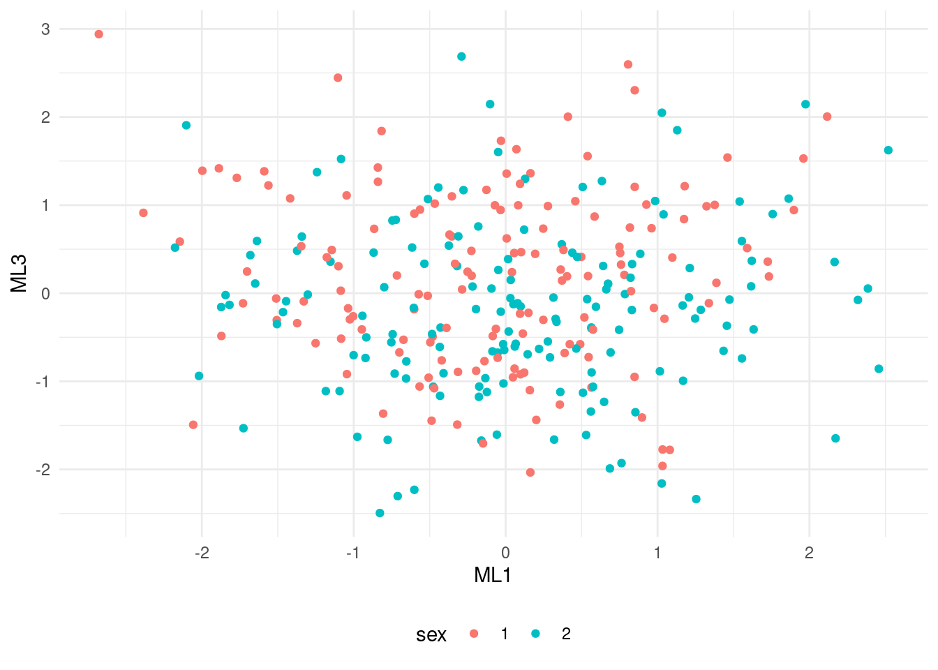

The plot show two uncorrelated factors, uniformly distributed among the two genders.

References

• Kaiser, H. F. (1974). An index of factor simplicity. Psychometrika, 39(1), 31-36.
• Statology (2019). A Guide to Bartlett’s Test of Sphericity. https://www.statology.org/bartletts-test-of-sphericity/
• Factor rotation methods (varimax, quartimax, oblimin, etc.) - what do the names mean and what do the methods do? https://stats.stackexchange.com/questions/185216/factor-rotation-methods-varimax-quartimax-oblimin-etc-what-do-the-names

Session Info

## R version 4.2.2 Patched (2022-11-10 r83330)
## Platform: x86_64-pc-linux-gnu (64-bit)
## Running under: Linux Mint 21.1
## 
## Matrix products: default
## BLAS:   /usr/lib/x86_64-linux-gnu/blas/libblas.so.3.10.0
## LAPACK: /usr/lib/x86_64-linux-gnu/lapack/liblapack.so.3.10.0
## 
## locale:
##  [1] LC_CTYPE=es_ES.UTF-8       LC_NUMERIC=C              
##  [3] LC_TIME=es_ES.UTF-8        LC_COLLATE=es_ES.UTF-8    
##  [5] LC_MONETARY=es_ES.UTF-8    LC_MESSAGES=es_ES.UTF-8   
##  [7] LC_PAPER=es_ES.UTF-8       LC_NAME=C                 
##  [9] LC_ADDRESS=C               LC_TELEPHONE=C            
## [11] LC_MEASUREMENT=es_ES.UTF-8 LC_IDENTIFICATION=C       
## 
## attached base packages:
## [1] stats     graphics  grDevices utils     datasets  methods   base     
## 
## other attached packages:
##  [1] kableExtra_1.3.4 lavaan_0.6-14    psych_2.2.9      corrr_0.4.4     
##  [5] forcats_0.5.2    stringr_1.5.0    dplyr_1.0.10     purrr_1.0.1     
##  [9] readr_2.1.3      tidyr_1.3.0      tibble_3.1.8     ggplot2_3.4.0   
## [13] tidyverse_1.3.2 
## 
## loaded via a namespace (and not attached):
##  [1] nlme_3.1-162        fs_1.6.0            lubridate_1.9.1    
##  [4] webshot_0.5.4       httr_1.4.4          tools_4.2.2        
##  [7] backports_1.4.1     bslib_0.4.2         utf8_1.2.2         
## [10] R6_2.5.1            DBI_1.1.3           colorspace_2.1-0   
## [13] withr_2.5.0         tidyselect_1.2.0    mnormt_2.1.1       
## [16] compiler_4.2.2      cli_3.6.0           rvest_1.0.3        
## [19] TSP_1.2-2           xml2_1.3.3          labeling_0.4.2     
## [22] bookdown_0.32       sass_0.4.5          scales_1.2.1       
## [25] quadprog_1.5-8      systemfonts_1.0.4   digest_0.6.31      
## [28] pbivnorm_0.6.0      rmarkdown_2.20      svglite_2.1.1      
## [31] ca_0.71.1           pkgconfig_2.0.3     htmltools_0.5.4    
## [34] dbplyr_2.3.0        fastmap_1.1.0       highr_0.10         
## [37] rlang_1.0.6         readxl_1.4.1        rstudioapi_0.14    
## [40] farver_2.1.1        jquerylib_0.1.4     generics_0.1.3     
## [43] jsonlite_1.8.4      googlesheets4_1.0.1 magrittr_2.0.3     
## [46] munsell_0.5.0       fansi_1.0.4         lifecycle_1.0.3    
## [49] stringi_1.7.12      yaml_2.3.7          grid_4.2.2         
## [52] parallel_4.2.2      crayon_1.5.2        lattice_0.20-45    
## [55] haven_2.5.1         hms_1.1.2           knitr_1.42         
## [58] pillar_1.8.1        codetools_0.2-19    stats4_4.2.2       
## [61] reprex_2.0.2        glue_1.6.2          evaluate_0.20      
## [64] blogdown_1.16       modelr_0.1.10       vctrs_0.5.2        
## [67] tzdb_0.3.0          foreach_1.5.2       cellranger_1.1.0   
## [70] gtable_0.3.1        assertthat_0.2.1    cachem_1.0.6       
## [73] xfun_0.36           broom_1.0.3         googledrive_2.0.0  
## [76] viridisLite_0.4.1   gargle_1.2.1        seriation_1.4.1    
## [79] iterators_1.0.14    registry_0.5-1      timechange_0.2.0   
## [82] ellipsis_0.3.2