Machine learning algorithms are explainable when it is possible to track its internal processes: how they make decisions, which variables are using and how variables influence model results. These explanations must be understood not only by developers, but also by users or regulators.
In this post, I will present how we can make explainable decision trees and regression based predictive models. I will apply some of these models to a classification job, and present how can we make these models explainable.
I will use the tidymodels framework, the rpart.plot package to plot decision trees built with rpart, and the vip package for variable importance plots.
library(tidymodels)
library(rpart.plot)
library(vip)
The dataset used is cat_adoption. It contains data from a subset of the cats at the animal shelter in Long Beach, California, USA. The job consists in predicting the event variable. It is equal to one when the cat is being homed or returned to its original location (i.e., owner or community). It is equal to zero when the cat is being transferred to another shelter or dying.
cat_adoption## # A tibble: 2,257 × 20
## time event sex neutered intake_condition intake_type latitude longitude
## <dbl> <dbl> <fct> <fct> <fct> <fct> <dbl> <dbl>
## 1 17 1 male yes fractious owner_surren… 33.8 -118.
## 2 98 1 male yes normal stray 33.8 -118.
## 3 15 0 male yes ill_moderatete owner_surren… 33.8 -118.
## 4 72 1 female yes fractious owner_surren… 33.8 -118.
## 5 22 0 male yes normal owner_surren… 33.8 -118.
## 6 66 1 male yes normal owner_surren… 33.8 -118.
## 7 200 1 female yes other other 33.9 -118.
## 8 9 0 female yes normal owner_surren… 33.9 -118.
## 9 45 1 male yes ill_mild stray 33.8 -118.
## 10 38 1 male no ill_mild stray 33.9 -118.
## # ℹ 2,247 more rows
## # ℹ 12 more variables: black <int>, brown <int>, brown_tabby <int>,
## # calico <int>, cream <int>, gray <int>, gray_tabby <int>, orange <int>,
## # orange_tabby <int>, tan <int>, tortie <int>, white <int>To use tidymodels we need to code the target variable as a factor and make the first level the positive case. I have renamed the levels as returned (positive case) and transfered for clarity.
cat_adoption <- cat_adoption |>
  mutate(event = as.factor(event))

#renaming levels
levels(cat_adoption$event) <- c("transfered", "returned")

# reordering to set positive case first
cat_adoption <- cat_adoption |>
  mutate(event = factor(event, levels = c("returned", "transfered")))
Let’s examine the target variable:
cat_adoption |>
  ggplot(aes(event, y = after_stat(count/sum(count)))) +
  geom_bar() +
  labs(title = "Target Variable", x = NULL, y = NULL) +
  theme_minimal()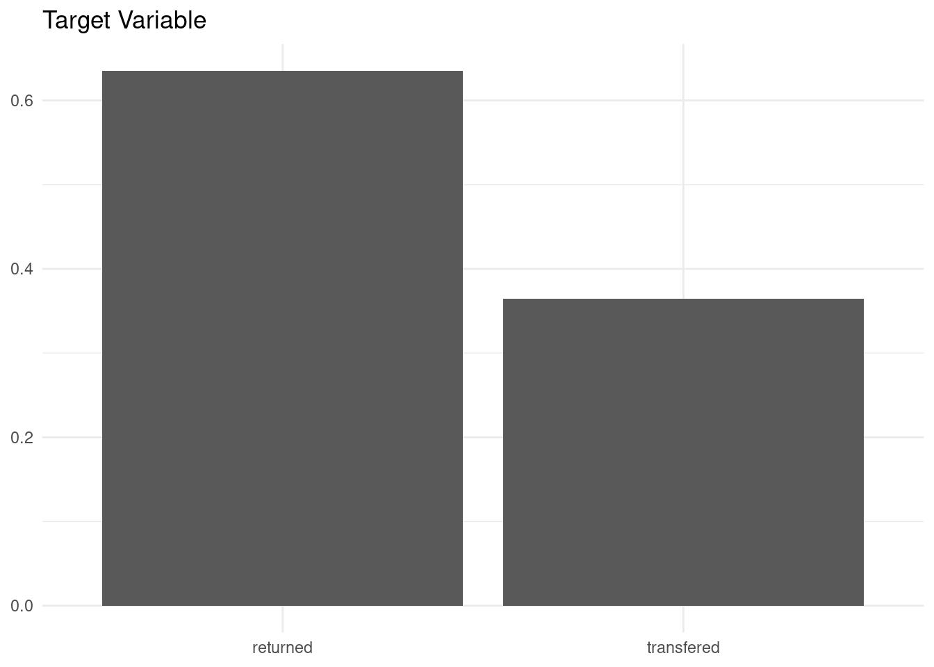
The positive case is more frequent than the negative, and the dataset seems balanced enough.
Decision Tree Models
Let’s start building two decision tree models. First, we need to split the sample into train and test:
set.seed(111)
split <- initial_split(cat_adoption, prop = 0.2, strata = "event")
The preprocessing recipe for decision tree models is quite simple: filtering non-zero and highly correlated variables, and exclude latitude and longitude.
rec_cats <- recipe(event ~ ., training(split)) |>
  step_rm(latitude:longitude) |>
  step_corr() |>
  step_nzv()
Now we can build two models:
- A decision tree
dtmodel withrpart. - A random forest model
rfwithranger. I have set the engine parameters to extract variable importance.
dt <- decision_tree(mode = "classification") |>
  set_engine("rpart")

rf <- rand_forest(mode = "classification") |>
  set_engine("ranger", importance = "impurity")
As the point here is to illustrate model explainability, I am training both models directly on the train set.
dt_model <- workflow() |>
  add_recipe(rec_cats) |>
  add_model(dt) |>
  fit(training(split))

rf_model <- workflow() |>
  add_recipe(rec_cats) |>
  add_model(rf) |>
  fit(training(split))
In the case of the decision tree model, we can see how the model has used variables to make the decision. I am using extract_fit_engine() to obtain the rpart output, and use this output to plot the decision tree with rpart.plot().
dt_model |>
  extract_fit_engine() |>
  rpart.plot(roundint = FALSE)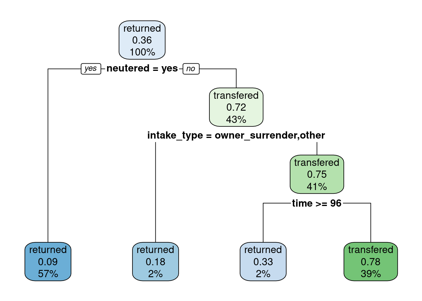
The most relevant variables in the model are neutered, intake_type and time. Specifically, neutered cats seem to have mode chances to be adopted than non-neutered.
Another important element to model transparency is variable importance. It is a measure of how useful or valuable each feature is in predicting the target variable. We can use vi() to obtain the raw values of variable importance, and vip() to do a variable importance plot.
vi(dt_model)## # A tibble: 7 × 2
## Variable Importance
## <chr> <dbl>
## 1 neutered 87.0
## 2 intake_condition 17.0
## 3 time 9.18
## 4 intake_type 6.80
## 5 sex 5.38
## 6 tortie 0.897
## 7 orange_tabby 0.449vip(dt_model) + theme_minimal() + ggtitle(label = "Variable Importance (Decision Tree).")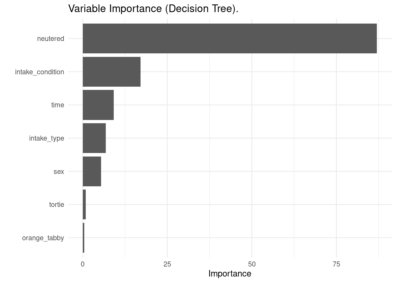
The variable importance analysis shows similar results to the decision tree plot: neutered, intake_condition and time are the most relevant variables for this model.
As the random forest algorithm uses a set of decision trees to make the decision, it is not possible to obtain a tree plot. But I can obtain variable importance plots with the vip() function.
vip(rf_model) + theme_minimal() + ggtitle(label = "Variable Importance (Random Forest).")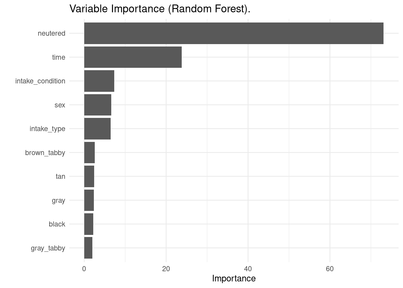
The most relevant variable is the same as with decision trees, but time, sex and some fur color variables are more relevant than intake type in random forests.
Regression Models
Let’s create two regression-based models: a straight linear logistic regression and a regularized regression model with glmnet. glmnet requires all variables to be numeric, so I will preprocess the factors accordingly.
rec_cats_lm <- recipe(event ~ ., training(split)) |>
  step_rm(latitude:longitude) |>
  step_nzv() |>
  step_corr() |>
  step_dummy(all_nominal_predictors())
Let’s test two logistic regression models: a glm model and a ridge (L2) model. Ridge regression models tend to shrink some coefficients, acting as an automated feature selector.
lr <- logistic_reg()

rr <- logistic_reg(penalty = 0.1, mixture = 0) |>
  set_engine("glmnet")
lr_model <- workflow() |>
add_recipe(rec_cats_lm) |>
add_model(lr) |>
fit(training(split))
rr_model <- workflow() |>
add_recipe(rec_cats_lm) |>
add_model(rr) |>
fit(training(split))We can obtain variable importance for each model with the vi() function. These variable importance factors are based on regression coefficients of variables. These coefficients can be positive or negative.
vi(lr_model)## # A tibble: 24 × 3
## Variable Importance Sign
## <chr> <dbl> <chr>
## 1 neutered_yes 10.3 NEG
## 2 time 2.88 NEG
## 3 tan 1.65 NEG
## 4 calico 1.59 NEG
## 5 intake_type_other 1.46 NEG
## 6 brown 1.40 POS
## 7 tortie 1.12 POS
## 8 white 0.979 NEG
## 9 intake_condition_other 0.769 NEG
## 10 gray_tabby 0.620 NEG
## # ℹ 14 more rowsvi(rr_model)## # A tibble: 25 × 3
## Variable Importance Sign
## <chr> <dbl> <chr>
## 1 neutered_yes 2.52 NEG
## 2 tan 1.53 NEG
## 3 intake_type_other 1.31 NEG
## 4 tortie 1.30 POS
## 5 calico 1.24 NEG
## 6 sex_unknown 1.23 POS
## 7 neutered_unknown 1.23 POS
## 8 brown 1.22 POS
## 9 white 0.599 NEG
## 10 orange 0.486 POS
## # ℹ 15 more rowsAlthough we can use the vip() function to build the plots, I will build them from the vi() tables.
library(forcats)
vi(lr_model) |>
  mutate(Variable = fct_reorder(Variable, Importance)) |>
  slice(1:10) |>
  ggplot(aes(Importance, Variable, fill = Sign)) +
  geom_col() +
  labs(title = "Variable importance (glm)", x = NULL, y = NULL) +
  theme_minimal() +
  theme(legend.position = "bottom")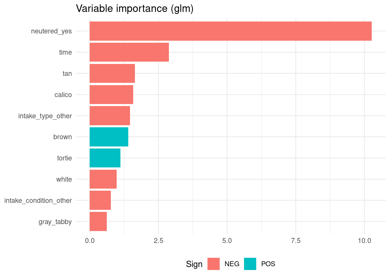
As the returned event is the first level of the target variable, negative regression terms are related with variables that increase the probability of the positive case.
vi(rr_model) |>
  mutate(Variable = fct_reorder(Variable, Importance)) |>
  slice(1:10) |>
  ggplot(aes(Importance, Variable, fill = Sign)) +
  geom_col() +
  labs(title = "Variable importance (glmnet)", x = NULL, y = NULL) +
  theme_minimal() +
  theme(legend.position = "bottom")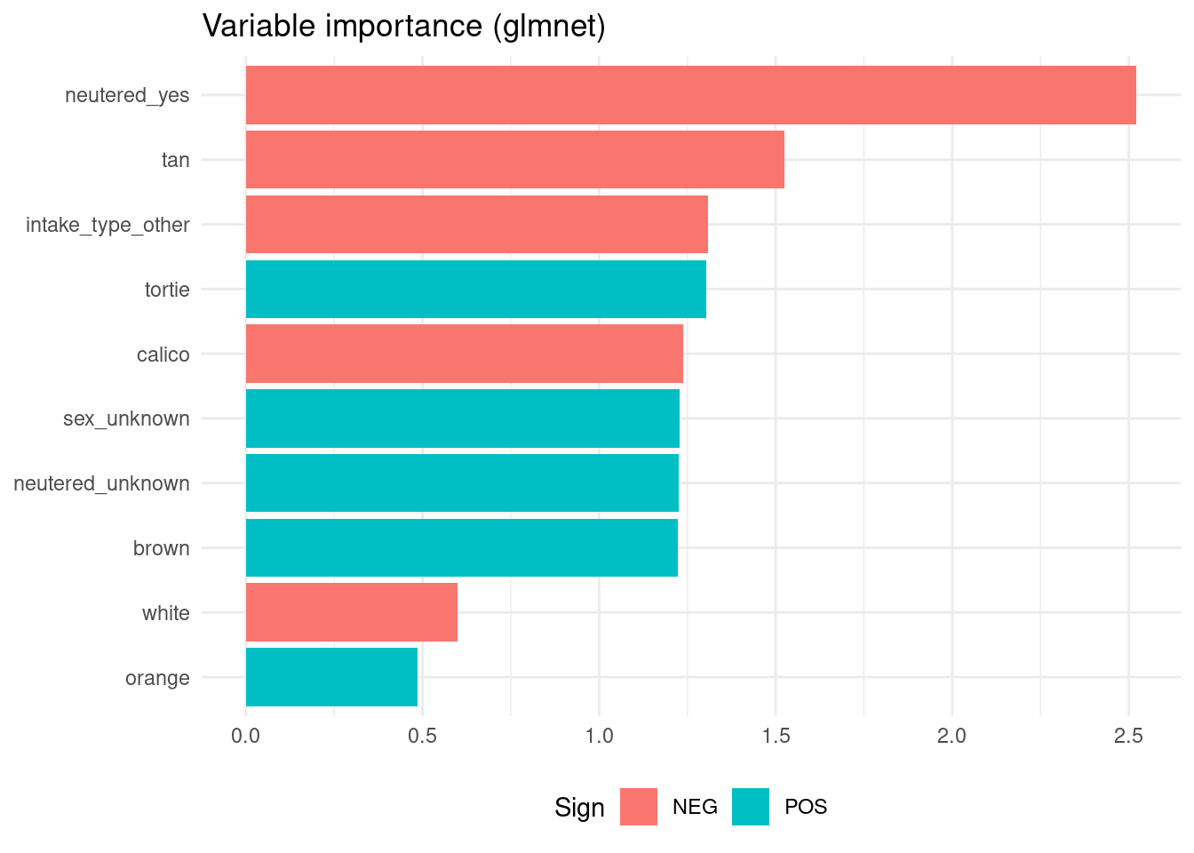
Contrarily to the other tree models, the glmnet model gives more importance to cat fur color.
Model Performance
Let’s evaluate the performance of the four models with cross validation. First I define the set of folds and the metrics used for model performance.
set.seed(111)
folds <- vfold_cv(training(split), v = 5)
cm <- metric_set(accuracy, sens, spec)
Then I am testing each model with cross validation, and aggregating all metrics in the performance_models tibble.
tree_models <- map2_dfr(list(dt, rf), c("dt", "rf"), ~
                     fit_resamples(object = .x,
                                   preprocessor = rec_cats,
                                   resamples = folds,
                                   metrics = cm) |>
                      collect_metrics() |>
                      mutate(mod = .y))

reg_models <- map2_dfr(list(lr, rr), c("lr", "rr"), ~
                     fit_resamples(object = .x,
                                   preprocessor = rec_cats_lm,
                                   resamples = folds,
                                   metrics = cm) |>
                      collect_metrics() |>
                      mutate(mod = .y))

performance_models <- rbind(tree_models, reg_models)

performance_models
## # A tibble: 12 × 7
## .metric .estimator mean n std_err .config mod
## <chr> <chr> <dbl> <int> <dbl> <chr> <chr>
## 1 accuracy binary 0.838 5 0.0156 Preprocessor1_Model1 dt
## 2 sens binary 0.847 5 0.0183 Preprocessor1_Model1 dt
## 3 spec binary 0.825 5 0.0298 Preprocessor1_Model1 dt
## 4 accuracy binary 0.831 5 0.0113 Preprocessor1_Model1 rf
## 5 sens binary 0.850 5 0.0145 Preprocessor1_Model1 rf
## 6 spec binary 0.800 5 0.0292 Preprocessor1_Model1 rf
## 7 accuracy binary 0.827 5 0.0152 Preprocessor1_Model1 lr
## 8 sens binary 0.840 5 0.0157 Preprocessor1_Model1 lr
## 9 spec binary 0.807 5 0.0425 Preprocessor1_Model1 lr
## 10 accuracy binary 0.824 5 0.0133 Preprocessor1_Model1 rr
## 11 sens binary 0.847 5 0.0152 Preprocessor1_Model1 rr
## 12 spec binary 0.789 5 0.0407 Preprocessor1_Model1 rrThe performance of the tree models is quite similar, but maybe the decision tree dt results to be the most explainable model with more balanced performance metrics between sensitivity and specificity.
We have made predictive models explainable through decision tree plots and variable importance plots. All models give great importance to the neutered variable, which seems to filter fairly enough positive and negative cases:
cat_adoption |>
  ggplot(aes(event, fill = neutered)) +
  geom_bar() +
  labs(title = "Neutered cats more likely to be returned", x = NULL, y = NULL) +
  theme_minimal() +
  theme(legend.position = "bottom")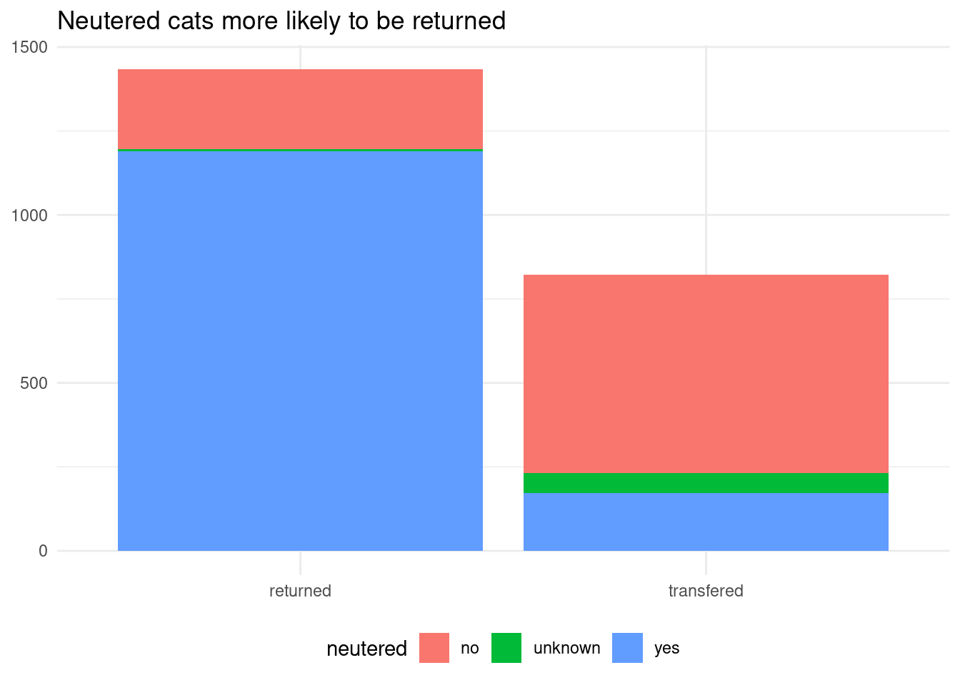
Reference
vip: variable importance plots: https://koalaverse.github.io/vip/index.html- Regularized regression with
glmnet: https://jmsallan.netlify.app/blog/regularized-regression-with-glmnet/ - Logistic regression via
glmnet: https://parsnip.tidymodels.org/reference/details_logistic_reg_glmnet.html
Session Info
## R version 4.5.0 (2025-04-11)
## Platform: x86_64-pc-linux-gnu
## Running under: Linux Mint 21.1
##
## Matrix products: default
## BLAS:   /usr/lib/x86_64-linux-gnu/blas/libblas.so.3.10.0
## LAPACK: /usr/lib/x86_64-linux-gnu/lapack/liblapack.so.3.10.0  LAPACK version 3.10.0
##
## locale:
##  [1] LC_CTYPE=es_ES.UTF-8       LC_NUMERIC=C
##  [3] LC_TIME=es_ES.UTF-8        LC_COLLATE=es_ES.UTF-8
##  [5] LC_MONETARY=es_ES.UTF-8    LC_MESSAGES=es_ES.UTF-8
##  [7] LC_PAPER=es_ES.UTF-8       LC_NAME=C
##  [9] LC_ADDRESS=C               LC_TELEPHONE=C
## [11] LC_MEASUREMENT=es_ES.UTF-8 LC_IDENTIFICATION=C
##
## time zone: Europe/Madrid
## tzcode source: system (glibc)
##
## attached base packages:
## [1] stats     graphics  grDevices utils     datasets  methods   base
##
## other attached packages:
##  [1] glmnet_4.1-8       Matrix_1.7-3       ranger_0.17.0      forcats_1.0.0
##  [5] vip_0.4.1          rpart.plot_3.1.2   rpart_4.1.24       yardstick_1.3.2
##  [9] workflowsets_1.1.0 workflows_1.2.0    tune_1.3.0         tidyr_1.3.1
## [13] tibble_3.2.1       rsample_1.3.0      recipes_1.3.0      purrr_1.0.4
## [17] parsnip_1.3.1      modeldata_1.4.0    infer_1.0.8        ggplot2_3.5.2
## [21] dplyr_1.1.4        dials_1.4.0        scales_1.3.0       broom_1.0.8
## [25] tidymodels_1.3.0
##
## loaded via a namespace (and not attached):
##  [1] tidyselect_1.2.1    timeDate_4041.110   farver_2.1.2
##  [4] fastmap_1.2.0       blogdown_1.21       digest_0.6.37
##  [7] timechange_0.3.0    lifecycle_1.0.4     survival_3.8-3
## [10] magrittr_2.0.3      compiler_4.5.0      rlang_1.1.6
## [13] sass_0.4.10         tools_4.5.0         utf8_1.2.4
## [16] yaml_2.3.10         data.table_1.17.0   knitr_1.50
## [19] labeling_0.4.3      DiceDesign_1.10     withr_3.0.2
## [22] nnet_7.3-20         grid_4.5.0          sparsevctrs_0.3.3
## [25] colorspace_2.1-1    future_1.40.0       globals_0.17.0
## [28] iterators_1.0.14    MASS_7.3-65         cli_3.6.4
## [31] rmarkdown_2.29      generics_0.1.3      rstudioapi_0.17.1
## [34] future.apply_1.11.3 cachem_1.1.0        splines_4.5.0
## [37] parallel_4.5.0      vctrs_0.6.5         hardhat_1.4.1
## [40] jsonlite_2.0.0      bookdown_0.43       listenv_0.9.1
## [43] foreach_1.5.2       gower_1.0.2         jquerylib_0.1.4
## [46] glue_1.8.0          parallelly_1.43.0   codetools_0.2-19
## [49] shape_1.4.6.1       lubridate_1.9.4     gtable_0.3.6
## [52] munsell_0.5.1       GPfit_1.0-9         pillar_1.10.2
## [55] furrr_0.3.1         htmltools_0.5.8.1   ipred_0.9-15
## [58] lava_1.8.1          R6_2.6.1            lhs_1.2.0
## [61] evaluate_1.0.3      lattice_0.22-5      backports_1.5.0
## [64] bslib_0.9.0         class_7.3-23        Rcpp_1.0.14
## [67] prodlim_2024.06.25  xfun_0.52           pkgconfig_2.0.3