Regularized regression

In datasets with many features, it can happen that using all of them leads to a worse performance than using only a subset. Selecting the features to introduce for better accuracy is the feature selection problem. There are two classical techniques of feature selection:

• Best subsets, which examines the fit of all possible subsets of features to choose the best subset. This can be computationally expensive. Sometimes we use algorithms like simulated annealing to choose that subset.
• Stepwise regression, consisting in adding or removing a feature in each step, until a satisfactory model is found.

An alternative to these strategies is regularization, in which we limit the total value of regression coefficients, so the regression coefficients of some variables shrink or go to zero.

The regression coefficients in the ordinary least squares (OLS) approach to linear regression are such that minimize the sum of squared errors:

\[ \displaystyle\sum_{i=1}^n \left( y_i - \hat{y}_i \right)^2 \]

Let’s examine two regularization approaches to OLS, lasso and ridge regression.

The name lasso stands for least absolute shrinkage and selection operator.

The approach of lasso is to force regression coefficients to shrink, forcing that the sum of absolute values or 1-norm to be smaller than a value \(t\):

\[ \displaystyle\sum_{j=1}^p |\beta_j| = \lVert \beta \lVert_1 \leq t\]

This is equivalent to minimizing:

\[ \displaystyle\sum_{i=1}^n \left( y_i - \hat{y}_i \right)^2 + \lambda \lVert \beta \lVert_1 \]

Lasso tends to set to zero some regression coefficients, so it works as an automated feature selection tool. As it uses the 1-norm of regression coefficients, lasso is also called L1 regularization.

Ridge regression uses a strategy analogous to lasso regression, but bounding the 2-norm (sum of squares) of the vector of regression coefficients to a value \(t\):

\[ \sqrt{\displaystyle\sum_{j=1}^p \beta_j^2} = \lVert \beta \lVert_2 \leq t \]

This is equivalent to minimizing:

\[ \displaystyle\sum_{i=1}^n \left( y_i - \hat{y}_i \right)^2 + \lambda \lVert \beta \lVert_2 \]

As ridge regression uses the 2-norm, we call it L2 regularization.

Ridge regression improves prediction error by shrinking coefficients of some variables.

We can mixt both regularizations in a mixed model introducing a mixture parameter which ranges from \(\alpha = 0\) for ridge regression and to \(\alpha = 1\) for lasso regression. \(\alpha\) is sometimes called the mixture parameter. These models are sometimes called elastic nets.

\[ \displaystyle\sum_{i=1}^n \left( y_i - \hat{y}_i \right)^2 + \lambda\left( \alpha \lVert \beta \lVert_2 + \left(1 - \alpha \right) \lVert \beta \lVert_1 \right) \]

The results of all these models depend on a \(\lambda\) parameter. As regularized regression is used mainly for prediction, we choose the value of lambda that best fits a prediction metric, usually the mean squared error. Let’s see how we can do that using glmnet.

A ridge regression model

glmnet requires entering variables in matrix format, that’s why I have generated dummies for categorical variables. I obtain the inputs to glmnet doing:

dep <- insurance %>%
  pull(charges)

vars <- insurance %>%
  select(-charges) %>%
  as.matrix()

Let’s obtain the ridge model:

ridge <- glmnet(x = vars, y = dep, alpha = 0)

glmnet has picked a range of values of \(\lambda\) and obtained the model for each. Let’s plot the evolution of coefficients with \(\lambda\):

plot(ridge, xvar = "lambda")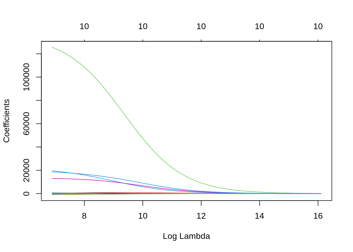

For high values of \(\lambda\), the coefficients of all variables are shrinking. Small values of \(\lambda\) result in coefficients similar to OLS. We need to select the value of \(\lambda\) for our prediction job as the one that minimizes a performance metric for prediction. cv.glmnet does that using cross validation.

cv_ridge <- cv.glmnet(x = vars,
                      y = dep,
                      alpha = 0)

Here are the results as a function of \(\lambda\):

plot(cv_ridge)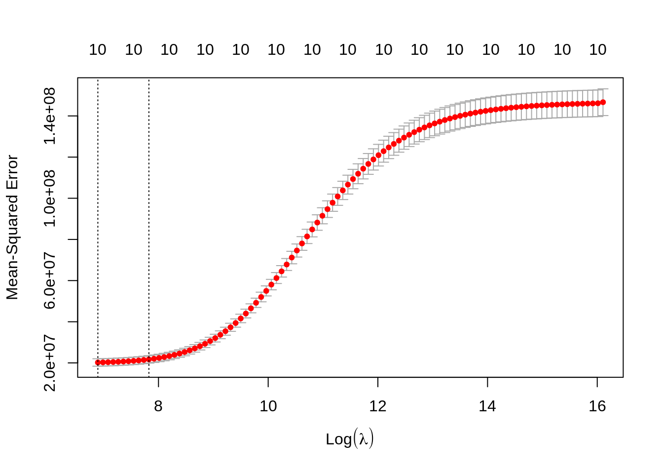

We get two values of \(\lambda\): the optimum lambda.min and lambda.1se which gives a similar fit with some more shrinking of coefficients. We obtain the values predicted with lambda.min doing:

pred_lambdamin_ridge <- predict(cv_ridge, 
                          s = cv_ridge$lambda.min, 
                          newx = vars)[, 1]

Lasso regression

To fit a lasso regression we set alpha = 1:

lasso <- glmnet(x = vars, y = dep, alpha = 1)

Let’s plot the evolution of coefficients:

plot(lasso, xvar = "lambda")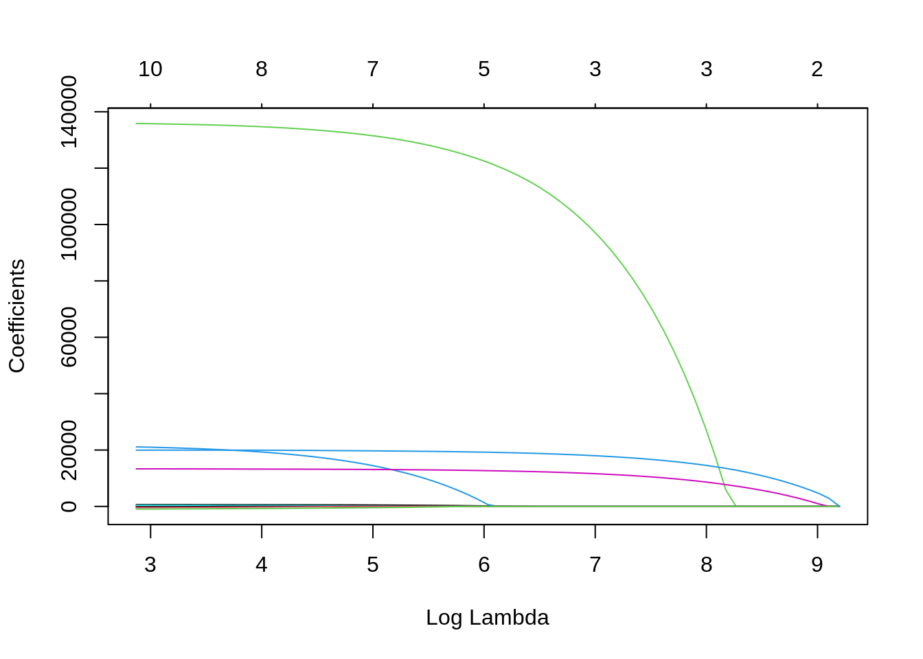

Lasso sets to zero coefficients of predictors as \(\lambda\) increases, so it can be considered an automated feature selector. The number of variables selected for each \(\lambda\) are presented in the scale above the plot. Let’s select \(\lambda\) with cross validation and plot the result:

cv_lasso <- cv.glmnet(x = vars,
                      y = dep,
                      alpha = 1,
                      penalty.factor = rep(1, 10))
plot(cv_lasso)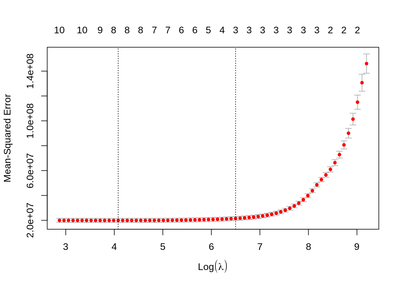

Finally, let’s do the prediction using lambda.min like in ridge regression.

pred_lambdamin_lasso <- predict(cv_lasso, 
                          s = cv_lasso$lambda.min, 
                          newx = vars)[, 1]

Model performance

I will use yardstick to evaluate performance of lasso and ridge regression. Let’s define a metric_set for numerical prediction.

np_metrics <- metric_set(rmse, mae, rsq)

Let’s store observed values and predictions in a data frame.

np_metrics <- metric_set(rmse, mae, rsq)
predictions <- tibble(real = dep,
                      ridge = pred_lambdamin_ridge,
                      lasso = pred_lambdamin_lasso) 

The performance of ridge regression:

predictions %>% 
  np_metrics(truth = real, estimate = ridge)

## # A tibble: 3 × 3
##   .metric .estimator .estimate
##   <chr>   <chr>          <dbl>
## 1 rmse    standard    4458.   
## 2 mae     standard    2574.   
## 3 rsq     standard       0.867

And the performance of lasso regression:

predictions %>% 
  np_metrics(truth = real, estimate = lasso)

## # A tibble: 3 × 3
##   .metric .estimator .estimate
##   <chr>   <chr>          <dbl>
## 1 rmse    standard    4423.   
## 2 mae     standard    2467.   
## 3 rsq     standard       0.867

Both models have quite similar performance in this case.

References

• Hastle, T., Qian, J., Tay, K. (2021). An introduction to glmnet. https://glmnet.stanford.edu/articles/glmnet.html
• Kaggle. Insurance premium prediction- https://www.kaggle.com/noordeen/insurance-premium-prediction
• Silge, Julia (2021). Add error for ridge regression with glmnet #431. https://github.com/tidymodels/parsnip/issues/431
• UC Business Analytics R Programming Guide. Regularized regression. https://uc-r.github.io/regularized_regression
• Yang, Y. (2021). Understand penalty.factor in glmnet. https://yuyangyy.medium.com/understand-penalty-factor-in-glmnet-9fb873f9045b

Session info

## R version 4.2.0 (2022-04-22)
## Platform: x86_64-pc-linux-gnu (64-bit)
## Running under: Linux Mint 19.2
## 
## Matrix products: default
## BLAS:   /usr/lib/x86_64-linux-gnu/openblas/libblas.so.3
## LAPACK: /usr/lib/x86_64-linux-gnu/libopenblasp-r0.2.20.so
## 
## locale:
##  [1] LC_CTYPE=es_ES.UTF-8       LC_NUMERIC=C              
##  [3] LC_TIME=es_ES.UTF-8        LC_COLLATE=es_ES.UTF-8    
##  [5] LC_MONETARY=es_ES.UTF-8    LC_MESSAGES=es_ES.UTF-8   
##  [7] LC_PAPER=es_ES.UTF-8       LC_NAME=C                 
##  [9] LC_ADDRESS=C               LC_TELEPHONE=C            
## [11] LC_MEASUREMENT=es_ES.UTF-8 LC_IDENTIFICATION=C       
## 
## attached base packages:
## [1] stats     graphics  grDevices utils     datasets  methods   base     
## 
## other attached packages:
## [1] glmnet_4.1-4     Matrix_1.4-1     BAdatasets_0.1.0 yardstick_0.0.9 
## [5] recipes_0.2.0    dplyr_1.0.9     
## 
## loaded via a namespace (and not attached):
##  [1] Rcpp_1.0.8.3       lubridate_1.8.0    lattice_0.20-45    tidyr_1.2.0       
##  [5] listenv_0.8.0      class_7.3-20       assertthat_0.2.1   digest_0.6.29     
##  [9] ipred_0.9-12       foreach_1.5.2      utf8_1.2.2         parallelly_1.31.1 
## [13] R6_2.5.1           plyr_1.8.7         hardhat_0.2.0      evaluate_0.15     
## [17] highr_0.9          blogdown_1.9       pillar_1.7.0       rlang_1.0.2       
## [21] rstudioapi_0.13    jquerylib_0.1.4    rpart_4.1.16       rmarkdown_2.14    
## [25] splines_4.2.0      gower_1.0.0        stringr_1.4.0      compiler_4.2.0    
## [29] xfun_0.30          pkgconfig_2.0.3    shape_1.4.6        globals_0.14.0    
## [33] htmltools_0.5.2    nnet_7.3-17        tidyselect_1.1.2   tibble_3.1.6      
## [37] prodlim_2019.11.13 bookdown_0.26      codetools_0.2-18   fansi_1.0.3       
## [41] future_1.25.0      crayon_1.5.1       withr_2.5.0        MASS_7.3-57       
## [45] grid_4.2.0         jsonlite_1.8.0     lifecycle_1.0.1    DBI_1.1.2         
## [49] magrittr_2.0.3     pROC_1.18.0        future.apply_1.9.0 cli_3.3.0         
## [53] stringi_1.7.6      timeDate_3043.102  bslib_0.3.1        ellipsis_0.3.2    
## [57] generics_0.1.2     vctrs_0.4.1        lava_1.6.10        iterators_1.0.14  
## [61] tools_4.2.0        glue_1.6.2         purrr_0.3.4        parallel_4.2.0    
## [65] fastmap_1.1.0      survival_3.2-13    yaml_2.3.5         knitr_1.39        
## [69] sass_0.4.1