In this post, I will introduce how to examine relationships between variables in a multivariate dataset using covariance and correlation matrices. Those matrices are the input of techniques like exploratory and confirmatory factor analysis and structural equation modelling. I this post, I will be using the mtcars dataset, that allows showing positive and negative relationships between variables.
In base R, we use cov and cor to obtain the covariances and correlation matrices of a multivariate distribution. These functions take a data frame with the observations as input.
c_mat <- cov(mtcars)
r_mat <- cor(mtcars)
The covariance matrix \(\mathbf{S}\) includes covariances \(s_{ij}\) between all pairs of variables \(\left(i, j\right)\) of the distribution. As \(s_{ij} = s_{ji}\), it is a symmetric matrix. Diagonal elements \(s_{ii}\) are the variance of each variable \(i\).
c_mat## mpg cyl disp hp drat wt
## mpg 36.324103 -9.1723790 -633.09721 -320.732056 2.19506351 -5.1166847
## cyl -9.172379 3.1895161 199.66028 101.931452 -0.66836694 1.3673710
## disp -633.097208 199.6602823 15360.79983 6721.158669 -47.06401915 107.6842040
## hp -320.732056 101.9314516 6721.15867 4700.866935 -16.45110887 44.1926613
## drat 2.195064 -0.6683669 -47.06402 -16.451109 0.28588135 -0.3727207
## wt -5.116685 1.3673710 107.68420 44.192661 -0.37272073 0.9573790
## qsec 4.509149 -1.8868548 -96.05168 -86.770081 0.08714073 -0.3054816
## vs 2.017137 -0.7298387 -44.37762 -24.987903 0.11864919 -0.2736613
## am 1.803931 -0.4657258 -36.56401 -8.320565 0.19015121 -0.3381048
## gear 2.135685 -0.6491935 -50.80262 -6.358871 0.27598790 -0.4210806
## carb -5.363105 1.5201613 79.06875 83.036290 -0.07840726 0.6757903
## qsec vs am gear carb
## mpg 4.50914919 2.01713710 1.80393145 2.1356855 -5.36310484
## cyl -1.88685484 -0.72983871 -0.46572581 -0.6491935 1.52016129
## disp -96.05168145 -44.37762097 -36.56401210 -50.8026210 79.06875000
## hp -86.77008065 -24.98790323 -8.32056452 -6.3588710 83.03629032
## drat 0.08714073 0.11864919 0.19015121 0.2759879 -0.07840726
## wt -0.30548161 -0.27366129 -0.33810484 -0.4210806 0.67579032
## qsec 3.19316613 0.67056452 -0.20495968 -0.2804032 -1.89411290
## vs 0.67056452 0.25403226 0.04233871 0.0766129 -0.46370968
## am -0.20495968 0.04233871 0.24899194 0.2923387 0.04637097
## gear -0.28040323 0.07661290 0.29233871 0.5443548 0.32661290
## carb -1.89411290 -0.46370968 0.04637097 0.3266129 2.60887097Covariance values depend on the scale of each pair of variables and thus they are difficult to interpret. That’s why we usually to examine the correlation matrix \(\mathbf{R}\). Correlations \(r_{ij}\) are scaled between -1 and +1, and diagonal elements are equal to one.
r_mat## mpg cyl disp hp drat wt
## mpg 1.0000000 -0.8521620 -0.8475514 -0.7761684 0.68117191 -0.8676594
## cyl -0.8521620 1.0000000 0.9020329 0.8324475 -0.69993811 0.7824958
## disp -0.8475514 0.9020329 1.0000000 0.7909486 -0.71021393 0.8879799
## hp -0.7761684 0.8324475 0.7909486 1.0000000 -0.44875912 0.6587479
## drat 0.6811719 -0.6999381 -0.7102139 -0.4487591 1.00000000 -0.7124406
## wt -0.8676594 0.7824958 0.8879799 0.6587479 -0.71244065 1.0000000
## qsec 0.4186840 -0.5912421 -0.4336979 -0.7082234 0.09120476 -0.1747159
## vs 0.6640389 -0.8108118 -0.7104159 -0.7230967 0.44027846 -0.5549157
## am 0.5998324 -0.5226070 -0.5912270 -0.2432043 0.71271113 -0.6924953
## gear 0.4802848 -0.4926866 -0.5555692 -0.1257043 0.69961013 -0.5832870
## carb -0.5509251 0.5269883 0.3949769 0.7498125 -0.09078980 0.4276059
## qsec vs am gear carb
## mpg 0.41868403 0.6640389 0.59983243 0.4802848 -0.55092507
## cyl -0.59124207 -0.8108118 -0.52260705 -0.4926866 0.52698829
## disp -0.43369788 -0.7104159 -0.59122704 -0.5555692 0.39497686
## hp -0.70822339 -0.7230967 -0.24320426 -0.1257043 0.74981247
## drat 0.09120476 0.4402785 0.71271113 0.6996101 -0.09078980
## wt -0.17471588 -0.5549157 -0.69249526 -0.5832870 0.42760594
## qsec 1.00000000 0.7445354 -0.22986086 -0.2126822 -0.65624923
## vs 0.74453544 1.0000000 0.16834512 0.2060233 -0.56960714
## am -0.22986086 0.1683451 1.00000000 0.7940588 0.05753435
## gear -0.21268223 0.2060233 0.79405876 1.0000000 0.27407284
## carb -0.65624923 -0.5696071 0.05753435 0.2740728 1.00000000There are many R packages dealing with correlation matrices, to allow a better visualization and interpretation. Here I will present some functionalities of corrr and corrplot packages.
library(corrr)
library(corrplot)
The corrr package
The corrr package is a part of the tidymodels ecosystem, and allows manipulating and presenting correlation matrices as data frames. We use correlate to obtain correlations with corrr.
r_df <- correlate(mtcars)The outcome of correlate is a tibble, instead of a matrix. Variable names of rows are stored in an additional term column. By default values of diagonal are set to NA.
r_df## # A tibble: 11 × 12
## term mpg cyl disp hp drat wt qsec vs am
## <chr> <dbl> <dbl> <dbl> <dbl> <dbl> <dbl> <dbl> <dbl> <dbl>
## 1 mpg NA -0.852 -0.848 -0.776 0.681 -0.868 0.419 0.664 0.600
## 2 cyl -0.852 NA 0.902 0.832 -0.700 0.782 -0.591 -0.811 -0.523
## 3 disp -0.848 0.902 NA 0.791 -0.710 0.888 -0.434 -0.710 -0.591
## 4 hp -0.776 0.832 0.791 NA -0.449 0.659 -0.708 -0.723 -0.243
## 5 drat 0.681 -0.700 -0.710 -0.449 NA -0.712 0.0912 0.440 0.713
## 6 wt -0.868 0.782 0.888 0.659 -0.712 NA -0.175 -0.555 -0.692
## 7 qsec 0.419 -0.591 -0.434 -0.708 0.0912 -0.175 NA 0.745 -0.230
## 8 vs 0.664 -0.811 -0.710 -0.723 0.440 -0.555 0.745 NA 0.168
## 9 am 0.600 -0.523 -0.591 -0.243 0.713 -0.692 -0.230 0.168 NA
## 10 gear 0.480 -0.493 -0.556 -0.126 0.700 -0.583 -0.213 0.206 0.794
## 11 carb -0.551 0.527 0.395 0.750 -0.0908 0.428 -0.656 -0.570 0.0575
## # … with 2 more variables: gear <dbl>, carb <dbl>With stretch we can get correlations as a long table:
stretch(r_df)## # A tibble: 121 × 3
## x y r
## <chr> <chr> <dbl>
## 1 mpg mpg NA
## 2 mpg cyl -0.852
## 3 mpg disp -0.848
## 4 mpg hp -0.776
## 5 mpg drat 0.681
## 6 mpg wt -0.868
## 7 mpg qsec 0.419
## 8 mpg vs 0.664
## 9 mpg am 0.600
## 10 mpg gear 0.480
## # … with 111 more rowsWith focus we can examine a part of the correlation matrix. Columns are the second argument of the function, and rows the rest of variables:
focus(r_df, c(mpg, cyl))## # A tibble: 9 × 3
## term mpg cyl
## <chr> <dbl> <dbl>
## 1 disp -0.848 0.902
## 2 hp -0.776 0.832
## 3 drat 0.681 -0.700
## 4 wt -0.868 0.782
## 5 qsec 0.419 -0.591
## 6 vs 0.664 -0.811
## 7 am 0.600 -0.523
## 8 gear 0.480 -0.493
## 9 carb -0.551 0.527fashion allows a pretty presentation of the correlation matrix. We can specify the number of decimals, and select if we want to print the leading_zeros. Here I am presenting the default input.
fashion(r_df)## term mpg cyl disp hp drat wt qsec vs am gear carb
## 1 mpg -.85 -.85 -.78 .68 -.87 .42 .66 .60 .48 -.55
## 2 cyl -.85 .90 .83 -.70 .78 -.59 -.81 -.52 -.49 .53
## 3 disp -.85 .90 .79 -.71 .89 -.43 -.71 -.59 -.56 .39
## 4 hp -.78 .83 .79 -.45 .66 -.71 -.72 -.24 -.13 .75
## 5 drat .68 -.70 -.71 -.45 -.71 .09 .44 .71 .70 -.09
## 6 wt -.87 .78 .89 .66 -.71 -.17 -.55 -.69 -.58 .43
## 7 qsec .42 -.59 -.43 -.71 .09 -.17 .74 -.23 -.21 -.66
## 8 vs .66 -.81 -.71 -.72 .44 -.55 .74 .17 .21 -.57
## 9 am .60 -.52 -.59 -.24 .71 -.69 -.23 .17 .79 .06
## 10 gear .48 -.49 -.56 -.13 .70 -.58 -.21 .21 .79 .27
## 11 carb -.55 .53 .39 .75 -.09 .43 -.66 -.57 .06 .27To interpret a correlation matrix, it can be useful to change the default order of variables, putting together highly correlated variables. We accomplish this with the rearrange function. The methods available to rearrange variables are principal components analysis "PCA" (the default) or hierarchical clustering "HC".
rearrange(r_df, method = "HC")## # A tibble: 11 × 12
## term wt cyl disp hp carb drat am gear qsec
## <chr> <dbl> <dbl> <dbl> <dbl> <dbl> <dbl> <dbl> <dbl> <dbl>
## 1 wt NA 0.782 0.888 0.659 0.428 -0.712 -0.692 -0.583 -0.175
## 2 cyl 0.782 NA 0.902 0.832 0.527 -0.700 -0.523 -0.493 -0.591
## 3 disp 0.888 0.902 NA 0.791 0.395 -0.710 -0.591 -0.556 -0.434
## 4 hp 0.659 0.832 0.791 NA 0.750 -0.449 -0.243 -0.126 -0.708
## 5 carb 0.428 0.527 0.395 0.750 NA -0.0908 0.0575 0.274 -0.656
## 6 drat -0.712 -0.700 -0.710 -0.449 -0.0908 NA 0.713 0.700 0.0912
## 7 am -0.692 -0.523 -0.591 -0.243 0.0575 0.713 NA 0.794 -0.230
## 8 gear -0.583 -0.493 -0.556 -0.126 0.274 0.700 0.794 NA -0.213
## 9 qsec -0.175 -0.591 -0.434 -0.708 -0.656 0.0912 -0.230 -0.213 NA
## 10 mpg -0.868 -0.852 -0.848 -0.776 -0.551 0.681 0.600 0.480 0.419
## 11 vs -0.555 -0.811 -0.710 -0.723 -0.570 0.440 0.168 0.206 0.745
## # … with 2 more variables: mpg <dbl>, vs <dbl>Correlation matrices are symmetric and with ones in the diagonal, so it is frequent to present its lower triangular part without diagonal elements. We get this with shave:
shave(r_df)## # A tibble: 11 × 12
## term mpg cyl disp hp drat wt qsec vs am gear
## <chr> <dbl> <dbl> <dbl> <dbl> <dbl> <dbl> <dbl> <dbl> <dbl> <dbl>
## 1 mpg NA NA NA NA NA NA NA NA NA NA
## 2 cyl -0.852 NA NA NA NA NA NA NA NA NA
## 3 disp -0.848 0.902 NA NA NA NA NA NA NA NA
## 4 hp -0.776 0.832 0.791 NA NA NA NA NA NA NA
## 5 drat 0.681 -0.700 -0.710 -0.449 NA NA NA NA NA NA
## 6 wt -0.868 0.782 0.888 0.659 -0.712 NA NA NA NA NA
## 7 qsec 0.419 -0.591 -0.434 -0.708 0.0912 -0.175 NA NA NA NA
## 8 vs 0.664 -0.811 -0.710 -0.723 0.440 -0.555 0.745 NA NA NA
## 9 am 0.600 -0.523 -0.591 -0.243 0.713 -0.692 -0.230 0.168 NA NA
## 10 gear 0.480 -0.493 -0.556 -0.126 0.700 -0.583 -0.213 0.206 0.794 NA
## 11 carb -0.551 0.527 0.395 0.750 -0.0908 0.428 -0.656 -0.570 0.0575 0.274
## # … with 1 more variable: carb <dbl>We can achieve a more satisfying presentation combining shave and fashion:
fashion(shave(r_df))## term mpg cyl disp hp drat wt qsec vs am gear carb
## 1 mpg
## 2 cyl -.85
## 3 disp -.85 .90
## 4 hp -.78 .83 .79
## 5 drat .68 -.70 -.71 -.45
## 6 wt -.87 .78 .89 .66 -.71
## 7 qsec .42 -.59 -.43 -.71 .09 -.17
## 8 vs .66 -.81 -.71 -.72 .44 -.55 .74
## 9 am .60 -.52 -.59 -.24 .71 -.69 -.23 .17
## 10 gear .48 -.49 -.56 -.13 .70 -.58 -.21 .21 .79
## 11 carb -.55 .53 .39 .75 -.09 .43 -.66 -.57 .06 .27We can also plot the correlation matrix with rplot. It is customary to rearrange and shave the matrix before plotting:
r_pretty <- shave(rearrange(r_df))
rplot(r_pretty)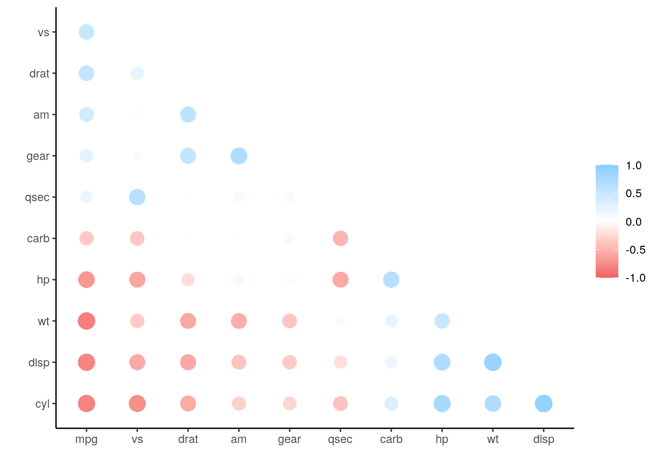
The corrplot package
corrplot provides a visual exploratory tool of correlation matrices that supports automatic variable reordering to help detect hidden patterns among variables. It can be seen as a visual alternative to exploratory factor analysis.
The functionalities of corrplot are nicely explained in the package vignette. Here I will be posting some illustrative examples.
We specify how to present correlations with the method argument of the corrplot function:
corrplot(r_mat, method = 'number') 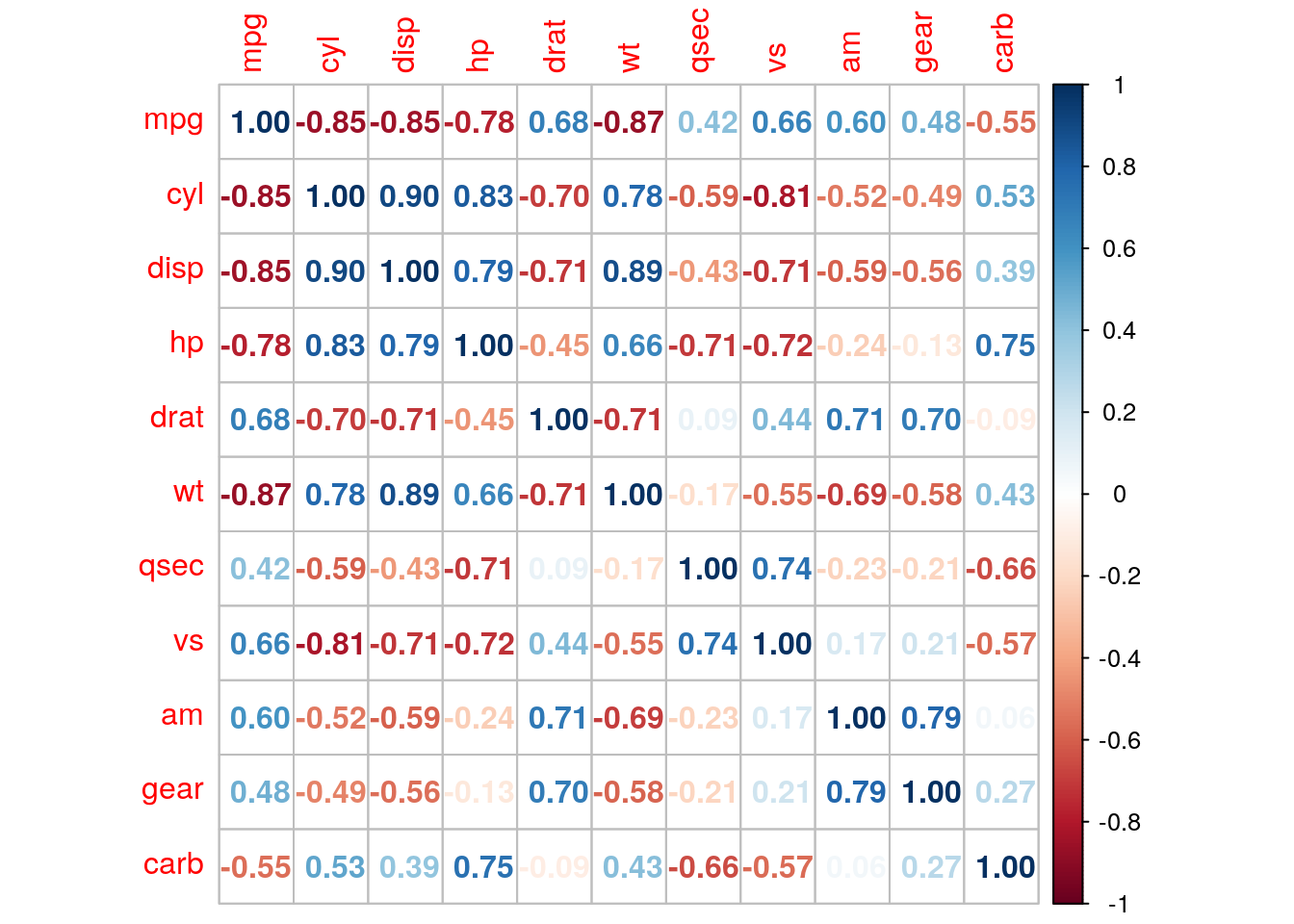
We can specify how to order variables in the correlation matrix. Methods available are angular order of eigenvectors "AOE", principal components "FPC" and hierarchical clustering "HC".
corrplot(r_mat, method = "circle", order = "hclust", diag = FALSE)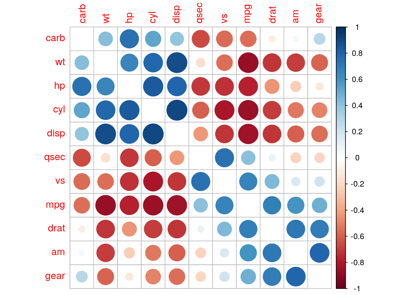
The corrplot.mixed function allows presenting two different visualizations of the same correlation matrix in the upper and lower triangular parts of the matrix.
corrplot.mixed(r_mat, upper = 'ellipse', lower = "shade", order = "hclust")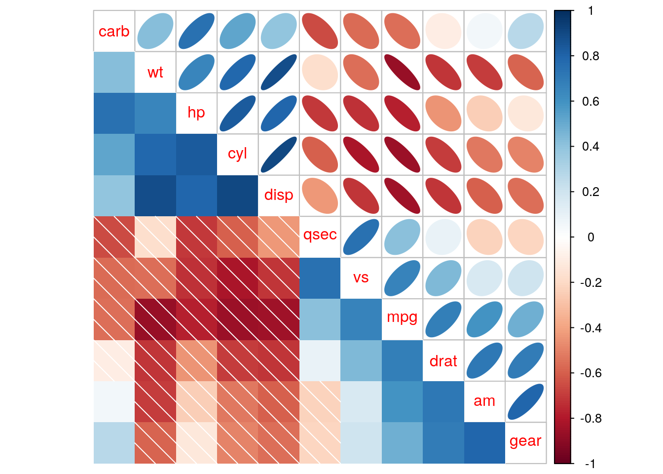
Examining covariance and correlation matrices in R
Covariance and correlation matrices express relationships between variables of a multivariate sample. As correlations are scaled between -1 nd +1, it is more convenient for humans to examine correlation matrices. With corrr and corrplot packages we can examine correlation matrices, group highly correlated subsets of variables and present visualizations of the results.
After examining correlation matrices, we can engage in advanced techniques to examine correlational structures, like exploratory and confirmatory factor analysis or structural equation modelling.
References
- Covariance and Pearson correlation in R https://jmsallan.netlify.app/blog/covariance-and-pearson-correlation-in-r/
corrrvignette: https://corrr.tidymodels.org/corrplotvignette: https://cran.r-project.org/web/packages/corrplot/vignettes/corrplot-intro.html
Session info
## R version 4.1.2 (2021-11-01)
## Platform: x86_64-pc-linux-gnu (64-bit)
## Running under: Debian GNU/Linux 10 (buster)
##
## Matrix products: default
## BLAS:   /usr/lib/x86_64-linux-gnu/blas/libblas.so.3.8.0
## LAPACK: /usr/lib/x86_64-linux-gnu/lapack/liblapack.so.3.8.0
##
## locale:
##  [1] LC_CTYPE=es_ES.UTF-8       LC_NUMERIC=C
##  [3] LC_TIME=es_ES.UTF-8        LC_COLLATE=es_ES.UTF-8
##  [5] LC_MONETARY=es_ES.UTF-8    LC_MESSAGES=es_ES.UTF-8
##  [7] LC_PAPER=es_ES.UTF-8       LC_NAME=C
##  [9] LC_ADDRESS=C               LC_TELEPHONE=C
## [11] LC_MEASUREMENT=es_ES.UTF-8 LC_IDENTIFICATION=C
##
## attached base packages:
## [1] stats     graphics  grDevices utils     datasets  methods   base
##
## other attached packages:
## [1] corrplot_0.92 corrr_0.4.3
##
## loaded via a namespace (and not attached):
##  [1] highr_0.9         bslib_0.2.5.1     compiler_4.1.2    pillar_1.6.4
##  [5] jquerylib_0.1.4   iterators_1.0.13  tools_4.1.2       digest_0.6.27
##  [9] jsonlite_1.7.2    evaluate_0.14     lifecycle_1.0.0   tibble_3.1.5
## [13] gtable_0.3.0      pkgconfig_2.0.3   rlang_0.4.12      foreach_1.5.1
## [17] registry_0.5-1    rstudioapi_0.13   cli_3.0.1         DBI_1.1.1
## [21] yaml_2.2.1        seriation_1.3.1   blogdown_1.5      xfun_0.23
## [25] TSP_1.1-11        stringr_1.4.0     dplyr_1.0.7       knitr_1.33
## [29] generics_0.1.0    sass_0.4.0        vctrs_0.3.8       tidyselect_1.1.1
## [33] grid_4.1.2        glue_1.4.2        R6_2.5.0          fansi_0.5.0
## [37] rmarkdown_2.9     bookdown_0.24     farver_2.1.0      purrr_0.3.4
## [41] ggplot2_3.3.5     magrittr_2.0.1    codetools_0.2-18  scales_1.1.1
## [45] htmltools_0.5.1.1 ellipsis_0.3.2    assertthat_0.2.1  colorspace_2.0-1
## [49] labeling_0.4.2    utf8_1.2.1        stringi_1.7.3     munsell_0.5.0
## [53] crayon_1.4.1