Correlation and covariance are the two main measures to evaluate the association between two numeric variables. In this post, I will define both measures, give some clues to interpret them and describe a test of hypothesis of association between two variables. I will also introduce some R base functions related with covariances and correlations. I will be using the tidyverse packages to handle data and create plots.
we define the population covariance of variables \(x\) and \(y\):
\[ \sigma_{xy} = \frac{1}{N} \sum_{i=1}^N \left(x_i - \mu_x\right) \left(y_i - \mu_y\right) \]
The covariance of a variable with itself is the sample variance:
\[ \sigma_{xx} = \sigma^2_x = \frac{1}{N} \sum_{i=1}^N \left(x_i - \mu_x\right)^2 \]
Usually we don’t know the population means, and we need to estimate them with sample means. The sample covariance of variables \(x\) and \(y\):
\[ s_{xy} = \frac{1}{N-1} \sum_{i=1}^N \left(x_i - \bar{x}\right) \left(y_i - \bar{y} \right) \]
We proceed similarly with sample variance:
\[ s_{xx} = s^2_x = \frac{1}{N-1} \sum_{i=1}^N \left(x_i - \bar{x}\right)^2 \]
We divide by sample size minus one to obtain unbiased estimators of covariance and variance.
Covariance between two variables can be positive or negative, while variance is always positive. The sign of covariance gives us information about how both variables relate. Let’s see how with an example:
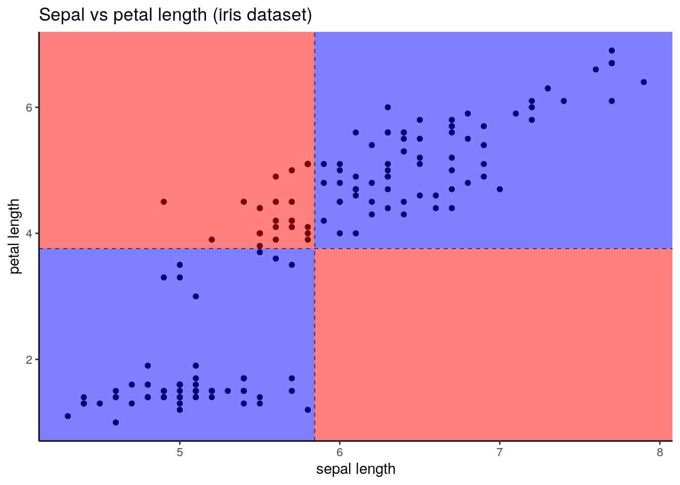
When centering (substracting the mean) of both variables, we can put each observation in one of the four zones. The ones in blue return a positive value of the product of centered variables, and the red return a negative value. If \(y\) tends to increase when \(x\) does, most observations will be in the blue zones, and the covariance will be positive. If it tends to decrease, most observations will be in the red zones, and the covariance will be negative. The same reasoning can be done with increases of \(y\), as covariance is a symmetric measure. In the example of the plot above, we can guees the covariance is positive. We use the R base cov function to confirm that:
## [1] 1.274315Covariance values depend on the units of the variables, so it can be hard to interpret the strength of the association. A remedy for this is to divide covariance by the standard deviation of both variables. This is equivalent to computing the covariance with standardized variables. The resulting measure is the Pearson correlation, abridged here to correlation. The expressions of the population \(\rho_{xy}\) and sample \(r_{xy}\) correlation are:
\[\begin{align} \rho_{xy} &= \frac{\sigma_{xy}}{\sigma_{x}\sigma_{y}} & r_{xy} &= \frac{s_{xy}}{s_xs_y} \end{align}\]
We use the R base cor function to calculate the correlation between two numerical vectors:
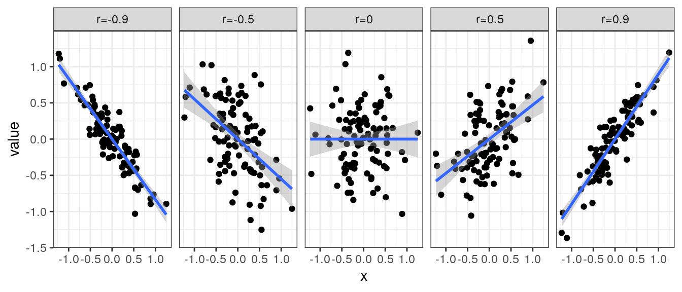
## [1] 0.8717538Correlations can take values between -1 and 1. Absolute values equal to one are sign of a perfect linear relationship, and a value of to zero indicates no association. In this plot I am presenting examples of five data sets with different values of correlation.
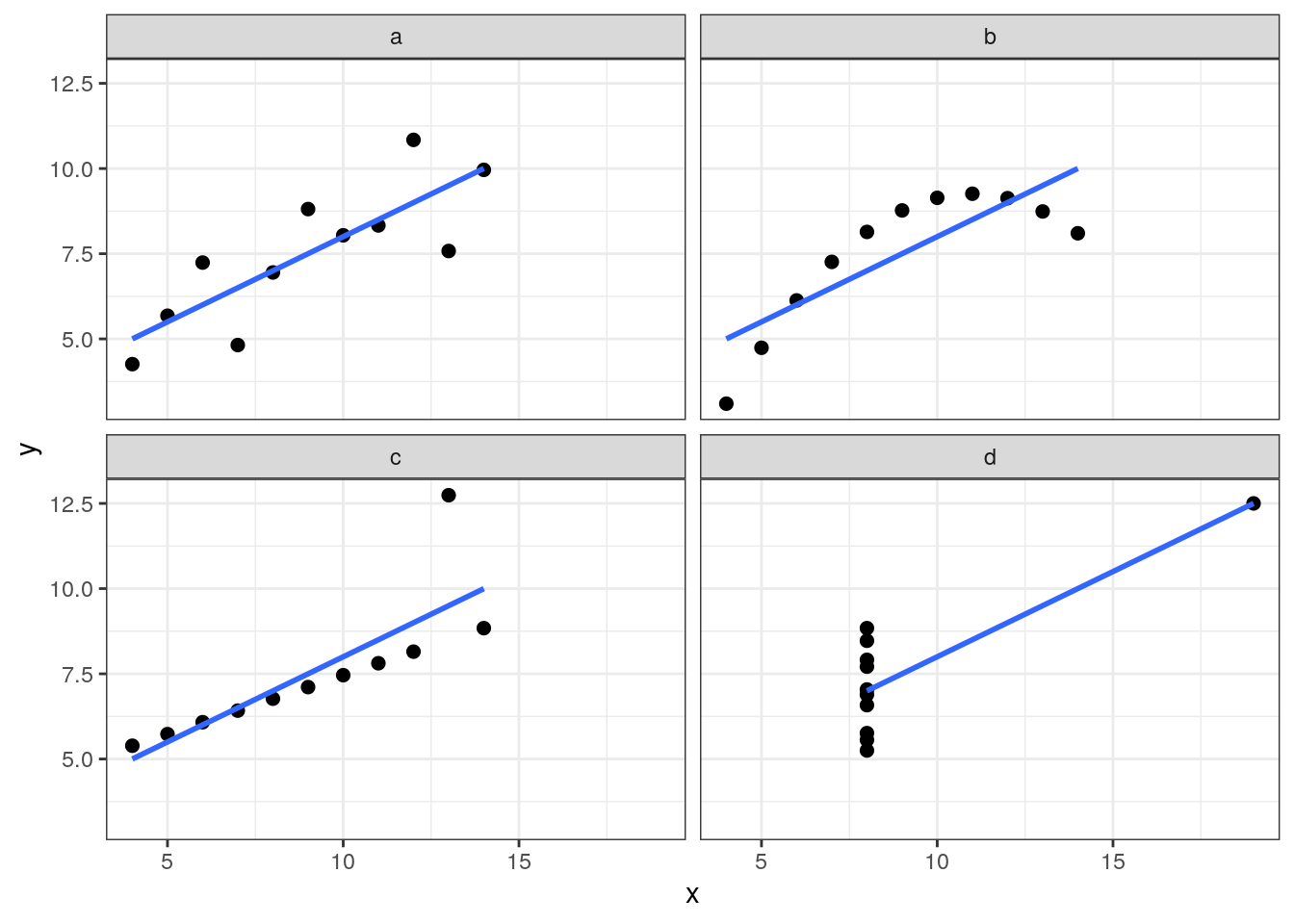
Correlation values give a partial view of the relationship between two variables, so it is important to examine bivariate plots when possible. An example of the dangers of relying on correlation alone are the data sets of the Anscombe (1973) quartet. The four data sets is in the anscombe variable of R base:
##    x1 x2 x3 x4    y1   y2    y3    y4
## 1  10 10 10  8  8.04 9.14  7.46  6.58
## 2   8  8  8  8  6.95 8.14  6.77  5.76
## 3  13 13 13  8  7.58 8.74 12.74  7.71
## 4   9  9  9  8  8.81 8.77  7.11  8.84
## 5  11 11 11  8  8.33 9.26  7.81  8.47
## 6  14 14 14  8  9.96 8.10  8.84  7.04
## 7   6  6  6  8  7.24 6.13  6.08  5.25
## 8   4  4  4 19  4.26 3.10  5.39 12.50
## 9  12 12 12  8 10.84 9.13  8.15  5.56
## 10  7  7  7  8  4.82 7.26  6.42  7.91
## 11  5  5  5  8  5.68 4.74  5.73  6.89
The four pairs of variables have similar values of correlation between each x and y:
## # A tibble: 4 × 3
##   set       n     r
##   <chr> <int> <dbl>
## 1 a        11 0.816
## 2 b        11 0.816
## 3 c        11 0.816
## 4 d        11 0.817
But a bivariate plot of each pair gives us a quite different picture of the relationship between variables:
Test of hypothesis for correlation
When examining a sample of two variables, we may ask if there is an association between them. We can answer this question making this null hypothesis on the population correlation:
\[ H_0: \rho = 0 \]
If \(H_0\) is true, the sample correlation \(r\) follows:
\[ \frac{r\sqrt{n-2}}{\sqrt{1-r^2}} \sim t_{N-2} \]
Making some algebra, we obtain the following expression that allows rejecting the null hypothesis with a confidence \(1-\alpha\), assuming a two-tailed test:
\[ |r| \geq \sqrt{\frac{t^2_{N-2, \alpha/2}}{N - 2 + t^2_{N-2, \alpha/2}}} \]
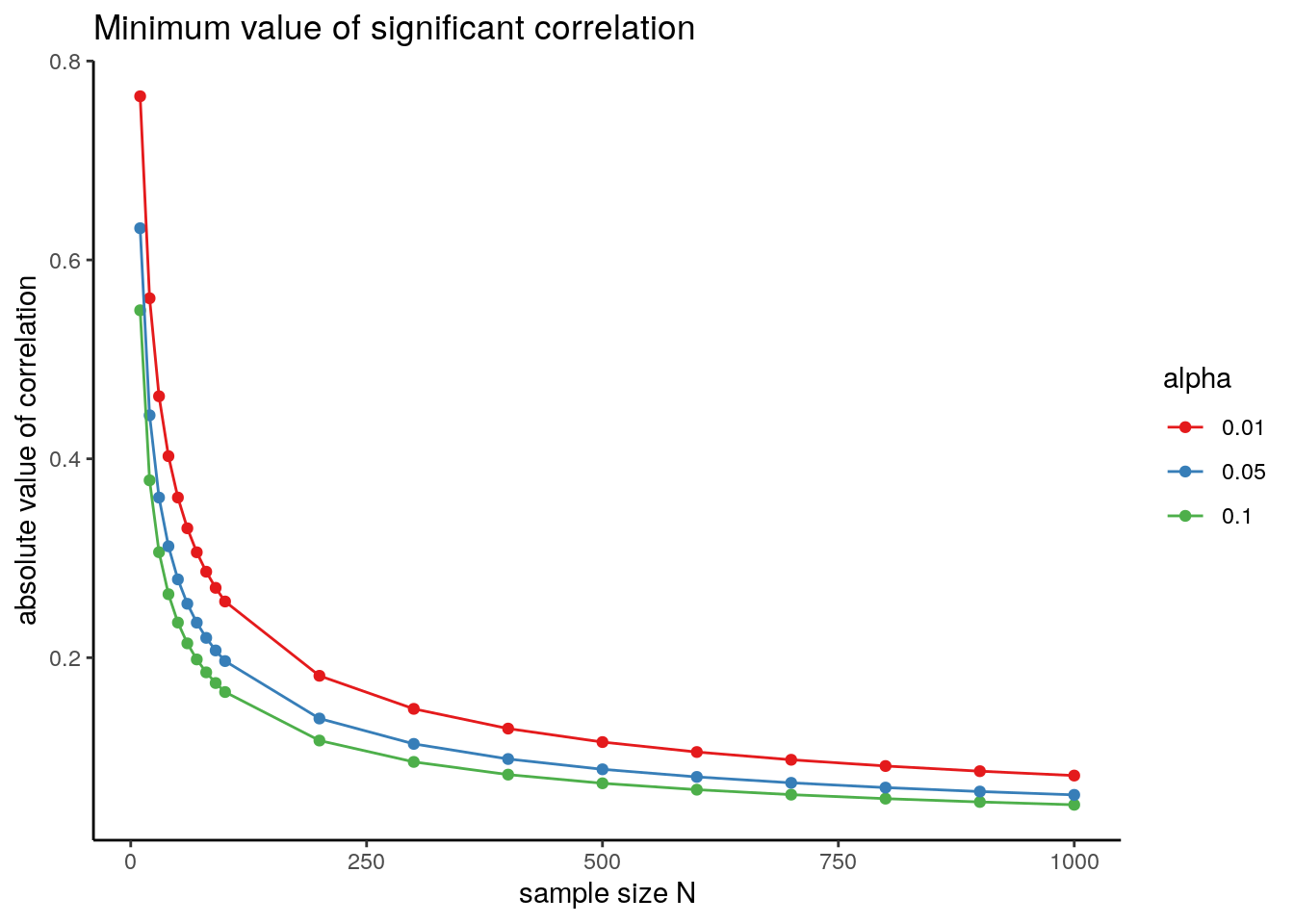
The minimum absolute value of correlation depends on sample size \(N\). Increasing sample size, we also increase the statistical power of the test. To detect weak associations between variables, we will need large sample sizes.
The plot below presents the minimum absolute value of correlation that can be considered significant for different values of sample size \(N\) and \(\alpha\):
We can perform the test of hypothesis for two variables using the cor.test function with the defaults (Pearson correlation, two-sided test). The function returns also a 95 percent confidence interval and the sample estimate.
##
##  Pearson's product-moment correlation
##
## data:  iris$Sepal.Length and iris$Petal.Length
## t = 21.646, df = 148, p-value < 2.2e-16
## alternative hypothesis: true correlation is not equal to 0
## 95 percent confidence interval:
##  0.8270363 0.9055080
## sample estimates:
##       cor
## 0.8717538
From the output of cor.test for these two variables, we learn that:
- The \(p\)-value is extremely low. This \(p\)-value is the probability of observing the obtained value or higher if the null hypothesis is true.
- The 95 percent interval does not include the zero.
As a consequence, it is safe to assume that the population correlation is different from zero in this case.
References
- Anscombe, F. J. (1973). Graphs in statistical analysis. The American statistician, 27(1), 17-21. https://doi.org/10.1080/00031305.1973.10478966
Built with R 4.1.1 and tidyverse 1.3.1