Creating Train and Test Sets

The aim of a predictive model is to perform well on unseen data, not used to train the model. To assess model performance, we need to split our dataset into two subsets:

• a train set of observations used to obtain (train) the model,
• a test set of observations that will be used to assess model performance.

Regarding train and test sets, we must take care that:

• the train and test sets must be representative of the same population,
• the test set must not be used to make any decision regarding the model, it must be used to assess model performance only.

We use the initial_split function to build the train and test sets:

• with p = 0.7 we set the 70% of observations in the train set,
• with strata = "medv" we perform stratified sampling so that the distribution of the target variable is similar to the whole sample in both sets.

As data splitting implies randomness, I have fixed the seed of the pseudo-random number generator to ensure reproducibility.

set.seed(1313)
bh_split <- initial_split(BostonHousing, prop = 0.7, strata = "medv")

Data Preprocessing

The recipe to pre process the dataset includes:

• the transformation of chas from factor to numeric with step_dummy. As the original chas value has only two levels, this steps generates a single dummy variable.
• looking for correlated predictors with step_corr, and for low-variability predictors with step_nzv.

bh_recipe <- training(bh_split) |>
  recipe(medv ~ .) |>
  step_dummy(chas) |>
  step_corr(all_predictors()) |>
  step_nzv(all_predictors())

We can see the results of applying the recipe doing prep():

bh_recipe |>
  prep()

## Recipe
## 
## Inputs:
## 
##       role #variables
##    outcome          1
##  predictor         13
## 
## Training data contained 352 data points and no missing data.
## 
## Operations:
## 
## Dummy variables from chas [trained]
## Correlation filter on tax [trained]
## Sparse, unbalanced variable filter removed <none> [trained]

The recipe is removing the tax variable, highly correlated with other variables:

Defining Models and Workflows

We will train two models:

• a linear regression model, using the R base lm function,
• a regression tree model, using the rpart package.

We will also define a workflow for each model so that we do the pre-processing with bh_recipe.

bh_lm <- linear_reg(mode = "regression") |>
  set_engine("lm")

bh_lm_wf <- workflow() |>
  add_recipe(bh_recipe) |>
  add_model(bh_lm)

bh_rt <- decision_tree(mode = "regression") |>
  set_engine("rpart")

bh_rt_wf <- workflow() |>
  add_recipe(bh_recipe) |>
  add_model(bh_rt)

Comparing Models with Cross Validation

We need to compare the performance of regression tree and linear regression models, preferably with a dataset different to the used to train the model to avoid overfitting. As we cannot make any decision about the model using the test set, we can use a cross validation strategy:

• randomly split the data into v folds f of approximately equal size,
• for each fold f, we train the data with the other f-1 folds and assess performance on f,
• optionally we repeat this repeats times,
• we average model performance across all folds and repeats.

We use the vfold_cv function to build the cross validation framework. I am defining three folds and three repeats, so we will perform nine evaluations of each model. With larger datasets, we can split the train set into more folders. We stratify by the dependent variable like in initial_split, so I am setting up againt the random number generator:

set.seed(1212)
bh_folds <- vfold_cv(training(bh_split), strata = "medv", v = 3, repeats = 3)

Model Performance Metrics

We will use three metrics to assess model performance. These metrics examine how close are predictions \(\hat{y}_i\) from observations \(y_i\) across all \(n\) observations.

The root mean square error rmse:

\[ \sqrt{\frac{\sum \left( \hat{y}_i - y_i \right)^2}{n}} \]

The mean absolute error mae:

\[ \frac{\sum \vert \hat{y}_i - y_i \vert}{n} \]

The coefficient of determination \(R^2\) rsq (where \(\bar{y}\) is the mean of \(y\)):

\[ 1- \frac{\sum \left( y_i - \hat{y}_i \right)^2}{\sum \left( y_i - \bar{y} \right)^2} \]

Good predictive models will have values of rmse and mae close to zero, and values of rsq close to one.

Let’s wrap the three metrics into a metrics_regression object with the metric_set function:

metrics_regression <- metric_set(rmse, mae, rsq)

Selecting a Model with Cross Validation

We use fit_resamples to evaluate each workflow with the cross validation scheme defined in bh_folds. The function will return the values of metrics_regression averaged across all folds and repeats.

The outputs have tibble format, so I am storing them and adding a column with the model description.

set.seed(1212)
lm_fit <- fit_resamples(bh_lm_wf, bh_folds, metrics = metrics_regression) |>
  collect_metrics() |>
  mutate(model = "lm")

set.seed(1212)
rt_fit <- fit_resamples(bh_rt_wf, bh_folds, metrics = metrics_regression) |>
  collect_metrics() |>
  mutate(model = "rt")

Let’s visualise the metrics for each model:

bind_rows(lm_fit, rt_fit) |>
  select(.metric, mean, std_err, model) |>
  ggplot(aes(x = model, y = mean, ymin = mean - 1.96*std_err, ymax = mean + 1.96*std_err)) +
  geom_pointrange() + 
  theme_bw() +
  labs(y = "confidence interval") +
  facet_grid(. ~ .metric)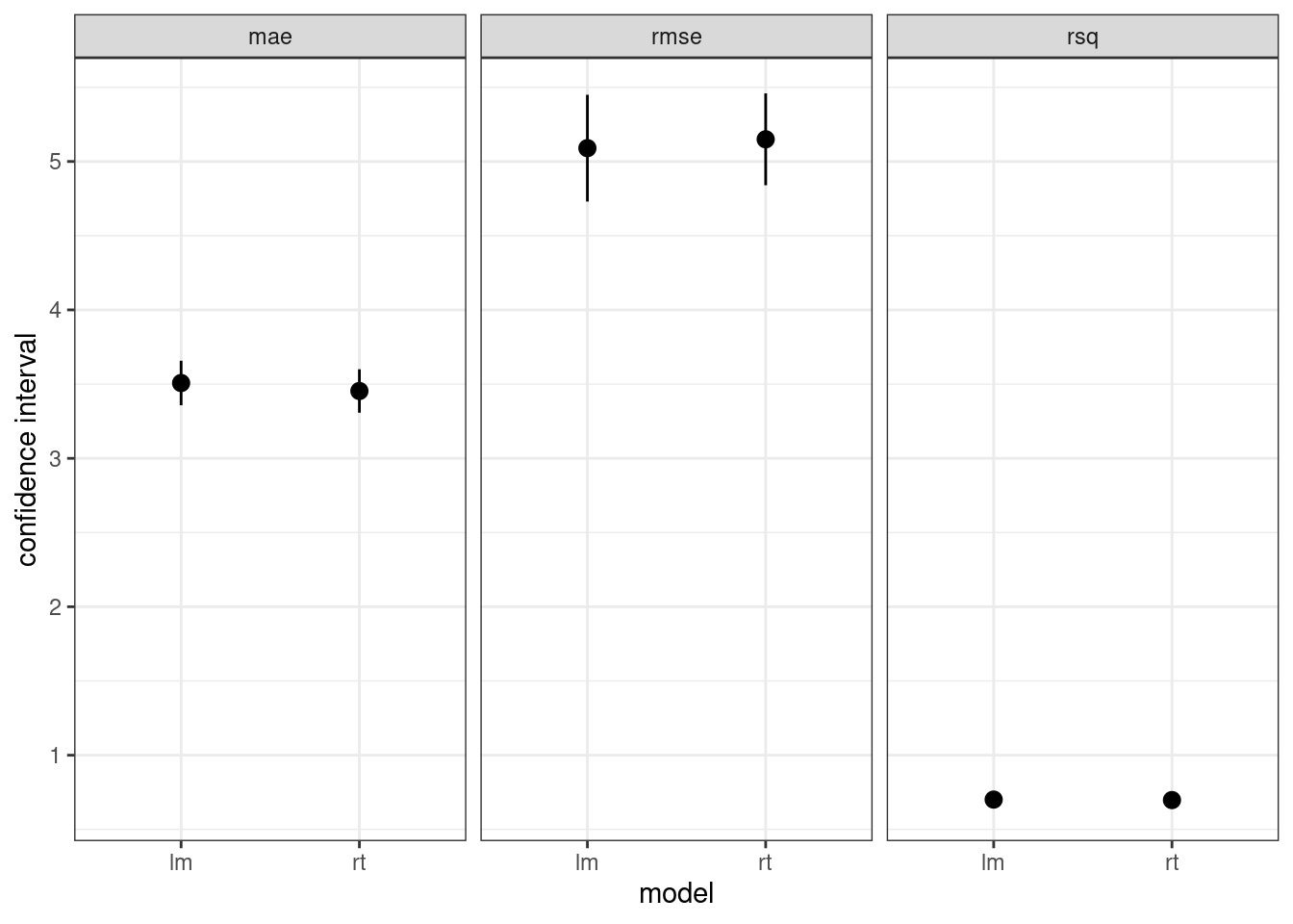

We observe that linear tree model has slightly better metrics than regression trees. Let’s present each of them in tabular form:

lm_fit |>
  select(model, .metric, mean, std_err)

## # A tibble: 3 × 4
##   model .metric  mean std_err
##   <chr> <chr>   <dbl>   <dbl>
## 1 lm    mae     3.51   0.0765
## 2 lm    rmse    5.09   0.183 
## 3 lm    rsq     0.701  0.0183

rt_fit |>
  select(model, .metric, mean, std_err)

## # A tibble: 3 × 4
##   model .metric  mean std_err
##   <chr> <chr>   <dbl>   <dbl>
## 1 rt    mae     3.45   0.0747
## 2 rt    rmse    5.15   0.158 
## 3 rt    rsq     0.698  0.0188

Fitting the Chosen Model with the Train set

We have chosen regression trees to predict data. Let’s fit the model to the whole train set:

fitted_model <- bh_lm_wf |>
  fit(training(bh_split))

And evaluate the metrics on the same train set:

predict_train <- fitted_model |>
  predict(training(bh_split)) |>
  bind_cols(training(bh_split)) |>
  mutate(sample = "train")

predict_train |>
  metrics_regression(truth = medv, estimate = .pred)

## # A tibble: 3 × 3
##   .metric .estimator .estimate
##   <chr>   <chr>          <dbl>
## 1 rmse    standard       4.74 
## 2 mae     standard       3.29 
## 3 rsq     standard       0.733

Evaluating Performance on the Test Set

To check the performance on unseen data, we need to evaluate performance on the test set:

predict_test <- fitted_model |>
  predict(testing(bh_split)) |>
  bind_cols(testing(bh_split)) |>
  mutate(sample = "test")

predict_test |>
  metrics_regression(truth = medv, estimate = .pred)

## # A tibble: 3 × 3
##   .metric .estimator .estimate
##   <chr>   <chr>          <dbl>
## 1 rmse    standard       4.85 
## 2 mae     standard       3.40 
## 3 rsq     standard       0.725

We observe that the metrics on the test set are worse than on the train set, so the chosen model has slight overfit.

We can also visualize the predicted vs real value for each dataset. Ideally, most of the dots of these plots should be over the dashed line of intercept zero and slope one.

bind_rows(predict_train, predict_test) |>
  ggplot(aes(medv, .pred)) +
  geom_point() +
  geom_abline(slope = 1, intercept = 0, size = 0.3, linetype = "dashed") +
  facet_grid(. ~ sample) +
  theme_bw()

## Warning: Using `size` aesthetic for lines was deprecated in ggplot2 3.4.0.
## ℹ Please use `linewidth` instead.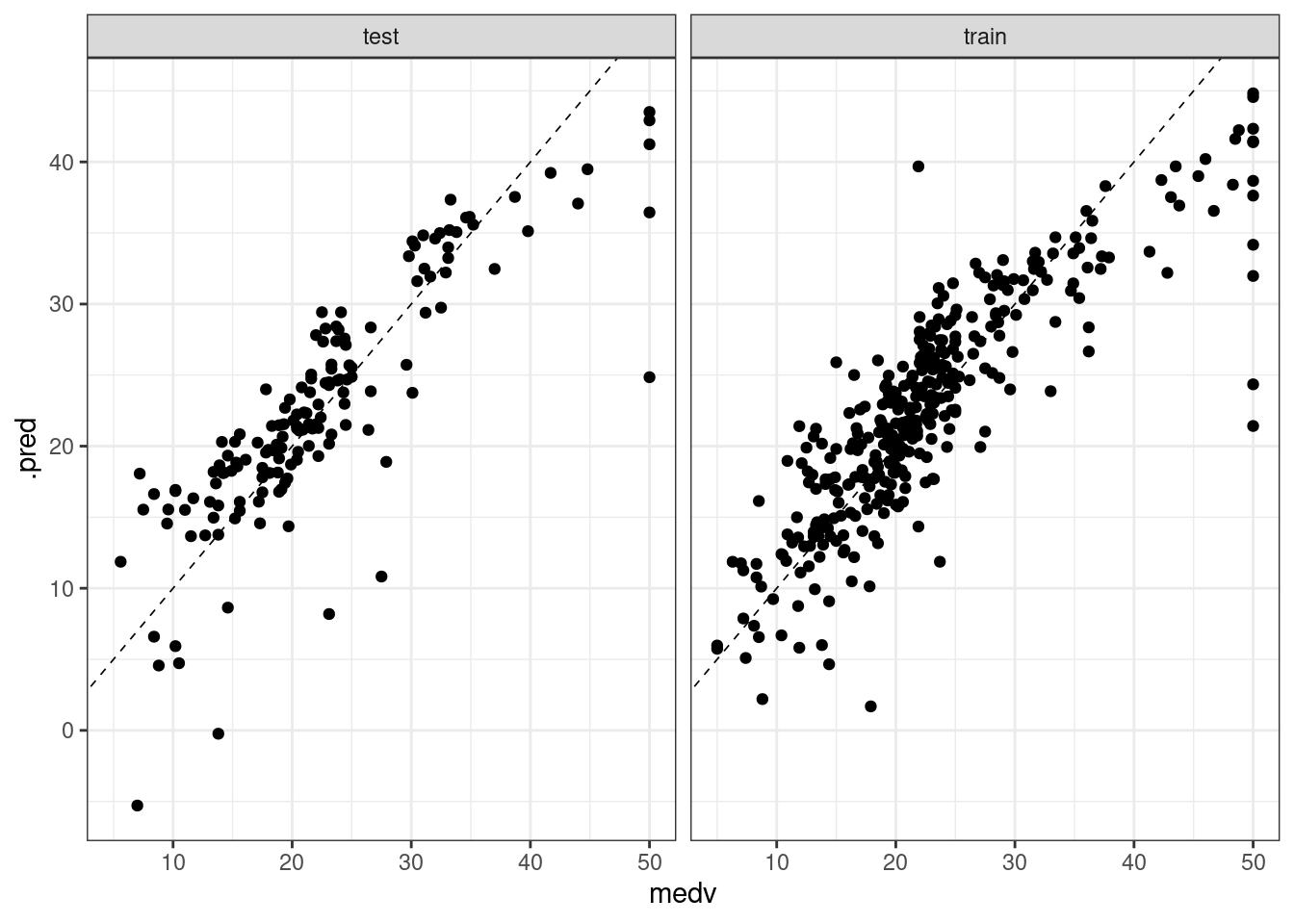

From the plots, we observe a similar pattern in the test and train sets.

References

• BostonHousing: Boston Housing Data https://rdrr.io/cran/mlbench/man/BostonHousing.html
• Harrison, D. and Rubinfeld, D.L. (1978). Hedonic prices and the demand for clean air. Journal of Environmental Economics and Management, 5, 81–102.
• Therneau, T. M. and Atkinson, E. J. (2019). An Introduction to Recursive Partitioning Using the RPART Routines. Available at: https://cran.r-project.org/web/packages/rpart/vignettes/longintro.pdf

Session Inof

## R version 4.2.2 Patched (2022-11-10 r83330)
## Platform: x86_64-pc-linux-gnu (64-bit)
## Running under: Linux Mint 21.1
## 
## Matrix products: default
## BLAS:   /usr/lib/x86_64-linux-gnu/blas/libblas.so.3.10.0
## LAPACK: /usr/lib/x86_64-linux-gnu/lapack/liblapack.so.3.10.0
## 
## locale:
##  [1] LC_CTYPE=es_ES.UTF-8       LC_NUMERIC=C              
##  [3] LC_TIME=es_ES.UTF-8        LC_COLLATE=es_ES.UTF-8    
##  [5] LC_MONETARY=es_ES.UTF-8    LC_MESSAGES=es_ES.UTF-8   
##  [7] LC_PAPER=es_ES.UTF-8       LC_NAME=C                 
##  [9] LC_ADDRESS=C               LC_TELEPHONE=C            
## [11] LC_MEASUREMENT=es_ES.UTF-8 LC_IDENTIFICATION=C       
## 
## attached base packages:
## [1] stats     graphics  grDevices utils     datasets  methods   base     
## 
## other attached packages:
##  [1] rpart_4.1.19       mlbench_2.1-3      yardstick_1.1.0    workflowsets_1.0.0
##  [5] workflows_1.1.2    tune_1.0.1         tidyr_1.3.0        tibble_3.1.8      
##  [9] rsample_1.1.1      recipes_1.0.4      purrr_1.0.1        parsnip_1.0.3     
## [13] modeldata_1.1.0    infer_1.0.4        ggplot2_3.4.0      dplyr_1.0.10      
## [17] dials_1.1.0        scales_1.2.1       broom_1.0.3        tidymodels_1.0.0  
## 
## loaded via a namespace (and not attached):
##  [1] sass_0.4.5          foreach_1.5.2       jsonlite_1.8.4     
##  [4] splines_4.2.2       prodlim_2019.11.13  bslib_0.4.2        
##  [7] assertthat_0.2.1    highr_0.10          GPfit_1.0-8        
## [10] yaml_2.3.7          globals_0.16.2      ipred_0.9-13       
## [13] pillar_1.8.1        backports_1.4.1     lattice_0.20-45    
## [16] glue_1.6.2          digest_0.6.31       hardhat_1.2.0      
## [19] colorspace_2.1-0    htmltools_0.5.4     Matrix_1.5-1       
## [22] timeDate_4022.108   pkgconfig_2.0.3     lhs_1.1.6          
## [25] DiceDesign_1.9      listenv_0.9.0       bookdown_0.32      
## [28] gower_1.0.1         lava_1.7.1          timechange_0.2.0   
## [31] farver_2.1.1        generics_0.1.3      ellipsis_0.3.2     
## [34] cachem_1.0.6        withr_2.5.0         furrr_0.3.1        
## [37] nnet_7.3-18         cli_3.6.0           survival_3.5-3     
## [40] magrittr_2.0.3      evaluate_0.20       future_1.31.0      
## [43] fansi_1.0.4         parallelly_1.34.0   MASS_7.3-58.2      
## [46] class_7.3-21        blogdown_1.16       tools_4.2.2        
## [49] lifecycle_1.0.3     munsell_0.5.0       compiler_4.2.2     
## [52] jquerylib_0.1.4     rlang_1.0.6         grid_4.2.2         
## [55] iterators_1.0.14    rstudioapi_0.14     labeling_0.4.2     
## [58] rmarkdown_2.20      gtable_0.3.1        codetools_0.2-19   
## [61] DBI_1.1.3           R6_2.5.1            lubridate_1.9.1    
## [64] knitr_1.42          fastmap_1.1.0       future.apply_1.10.0
## [67] utf8_1.2.2          parallel_4.2.2      Rcpp_1.0.10        
## [70] vctrs_0.5.2         tidyselect_1.2.0    xfun_0.36

Updated at 2023-03-20 10:34:04.