While I am publishing this post, the 2022 World Cup is taking place in Qatar. To celebrate this event, I will use the tidytuesday data about World Cups celebrated until 2018 to present two visualizations about the past winners of the World Cup. The packages I will be using are:
library(tidyverse)
library(ggimage)
library(kableExtra)
library(tidytuesdayR)
library(countrycode)
The tidyverse package loads utilties for data handling and visualization. ggimage allows placing images in plots done with gpplot2. I am using kableExtra to print tables.
I am using tidytuesdayR to load World Cup data from the Tidytuesday GitHub repository. countrycode allows obtaining data about countries, like the iso codes and the continent the country is in.
Let’s load the data about the world cup with tt_load. Here I will be using the worldcups dataset only.
tuesdata <- tidytuesdayR::tt_load(2022, week = 48)
wcmatches <- tuesdata$wcmatches
worldcups <- tuesdata$worldcups
rm(tuesdata)load("worldcup.RData")worldcups contains information about each edition World Cup, among them the year and the winner:
worldcups %>% glimpse()## Rows: 21
## Columns: 10
## $ year <dbl> 1930, 1934, 1938, 1950, 1954, 1958, 1962, 1966, 1970, 197…
## $ host <chr> "Uruguay", "Italy", "France", "Brazil", "Switzerland", "S…
## $ winner <chr> "Uruguay", "Italy", "Italy", "Uruguay", "West Germany", "…
## $ second <chr> "Argentina", "Czechoslovakia", "Hungary", "Brazil", "Hung…
## $ third <chr> "USA", "Germany", "Brazil", "Sweden", "Austria", "France"…
## $ fourth <chr> "Yugoslavia", "Austria", "Sweden", "Spain", "Uruguay", "W…
## $ goals_scored <dbl> 70, 70, 84, 88, 140, 126, 89, 89, 95, 97, 102, 146, 132, …
## $ teams <dbl> 13, 16, 15, 13, 16, 16, 16, 16, 16, 16, 16, 24, 24, 24, 2…
## $ games <dbl> 18, 17, 18, 22, 26, 35, 32, 32, 32, 38, 38, 52, 52, 52, 5…
## $ attendance <dbl> 434000, 395000, 483000, 1337000, 943000, 868000, 776000, …Winners of the World Cup (1930-2018)
Let’s see what countries have ever won a World Cup:
unique(worldcups$winner)## [1] "Uruguay" "Italy" "West Germany" "Brazil" "England"
## [6] "Argentina" "France" "Spain" "Germany"When it comes to football, West Germany is equivalent to Germany. Let’s replace their appearances in the table:
worldcups <- worldcups %>%
  mutate(winner = replace(winner, winner == "West Germany", "Germany"))
Let’s see how many Cups has won each country. I’ll store that information in the winners table.
winners <- worldcups %>%
  group_by(winner) %>%
  summarize(n = n(), .groups = "drop")

winners %>%
  kbl() %>%
kable_styling(full_width = FALSE)| winner | n |
|---|---|
| Argentina | 2 |
| Brazil | 5 |
| England | 1 |
| France | 2 |
| Germany | 4 |
| Italy | 4 |
| Spain | 1 |
| Uruguay | 2 |
The obvious way of visualizing this information is through a bar plot. Let’s see the default view:
winners %>%
  ggplot(aes(winner, n)) +
  geom_bar(stat = "identity")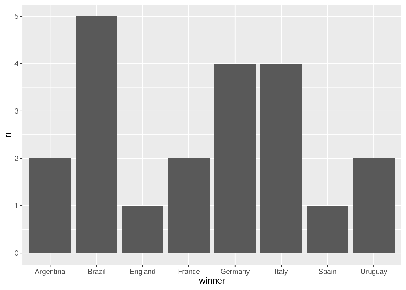
An edited barplot
Let’s do a better plot, ordering the bars, plotting each winner’s continent and presenting the countries with their flags. To do so, I’ve:
- Obtained the
iso2code andcontinentof each country. - As England is missing in the table, I am replacing its values, and picking a file with the English flag from the internet with
england_link.
winners <- winners %>%
  mutate(iso2 = countrycode(winner, "country.name", "iso2c"),
         continent = countrycode(winner, "country.name", "continent"))

winners <- winners %>%
  mutate(iso2 = replace(iso2, is.na(iso2), "EN"),
         continent = replace(continent, is.na(continent), "Europe"))

england_link <- "https://upload.wikimedia.org/wikipedia/en/thumb/b/be/Flag_of_England.svg/800px-Flag_of_England.svg.png"
Here is the new version of the visualization of the World Cup winners:
- Define the plot as a bar plot, with fill color defined by continent of each country.
- Set the limits of y axis with
ylimso that I can set the flags on the left hand side. - Placing country flags in
y = -0.5withgeom_flag. England flag is missing as it is not included in this geom. - Placing the English flag with
geom_image. - Placing the number of World Cups won of each country with
geom_textfor better readability. This will allow removing the y axis later. - Flip axis with
coord_flipand remove axis and background withtheme_void. - Set an image title with
ggtitle. - Tune colors and legend labels with
scale_fill_manual. Legend size is tuned withlegend.*parameters in thetheme. - Change title size with
plot.titleintheme.
winners %>%
  mutate(winner = fct_reorder(winner, n)) %>%
  ggplot(aes(winner, n, fill = continent)) +
  geom_bar(stat = "identity") +
  ylim(-1, 5) +
  geom_flag(y = -0.5, aes(image = iso2), size = 0.12) +
  geom_image(aes(x = "England", y = -0.5, image = england_link), size = 0.12) +
  geom_text(aes(label = n), hjust = -1, size = 5) +
  coord_flip() +
  theme_void() +
  ggtitle("Winners of the World Cup until 2018") +
  scale_fill_manual(values = c("#9E66AB", "#599AD3"), label = c("America", "Europe")) +
  theme(legend.position = c(0.7, 0.2),
        legend.key.size = unit(1, 'cm'),
        legend.text = element_text(size = 12),
        legend.title = element_text(size = 15),
        plot.title = element_text(size = 20))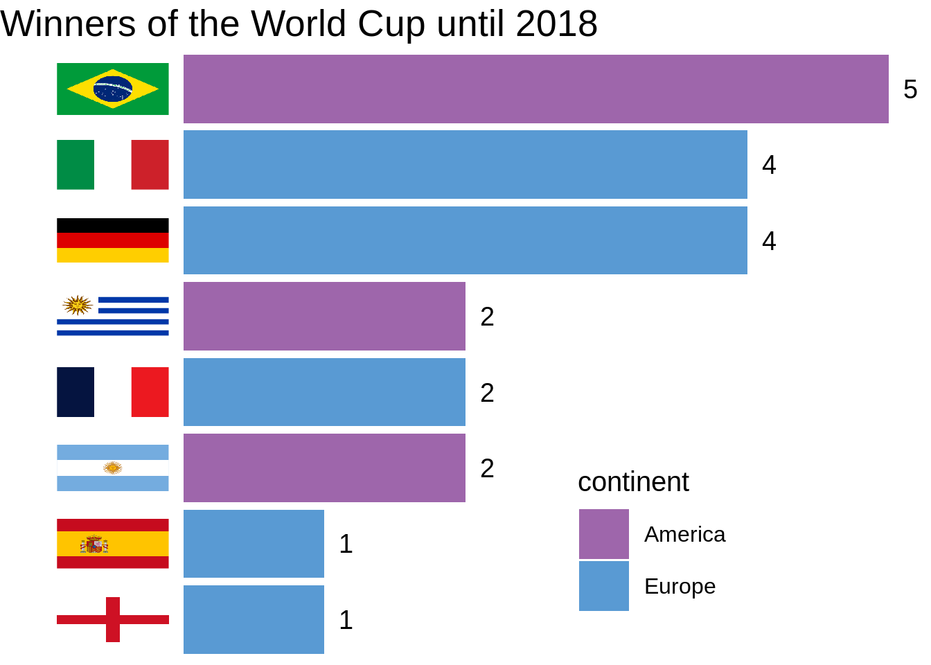
The resulting barplot is hopefully more informative than the default plot.
A World Cup winners timeline
I have also done a timeline plot presenting where has won the World Cups each of the winners. For doing that, I need to obtain World Cup winners ordered with non-increasing order of Cups won l_winners:
l_winners <- winners %>%
  arrange(n) %>%
  pull(winner)
I also need a the url address of a World Cup icon:
world_cup_icon <- "https://upload.wikimedia.org/wikipedia/commons/thumb/b/ba/FIFA_World_Cup_Icon_%28Campionato_mondiale_di_calcio%29.svg/94px-FIFA_World_Cup_Icon_%28Campionato_mondiale_di_calcio%29.svg.png"Here is the plot. Let’s see how I have done it:
- I am retrieving the
iso2country codes inworldcupsto set the flags later. - The plot has
yearin the x axis, andwinnerin the y axis. - In every year a country has won a World Cup I am placing a World Cup icon with
geom_image. - I am placing country flags on the left-hand size like in the previous plot. Let’s remember that first World Cup was celebrated in 1930. I am using
geom_flagandgeom_imagein the same was as in the previous plot. - I am changing the default labels of the
yearsaxis withscale_x_continuous. - I am using
theme_minimalto maintain the grid lines in a white background. InthemeI am removing all elements of the y axis.
worldcups %>%
  mutate(winner = factor(winner, levels = l_winners),
         iso2 = countrycode(winner, "country.name", "iso2c")) %>%
  mutate(iso2 = replace(iso2, is.na(iso2), "EN")) %>%
  ggplot(aes(year, winner)) +
  geom_image(image = world_cup_icon, size = 0.03) +
  geom_flag(x = 1920, aes(image = iso2)) +
  geom_image(aes(y = "England", x = 1920, image = england_link)) +
  scale_x_continuous(limits = c(1920, 2018), breaks = seq(1930, 2018, 8), name = element_blank()) +
  theme_minimal() +
  theme(axis.text.y = element_blank(),
        axis.ticks.y = element_blank(),
        axis.title.y = element_blank())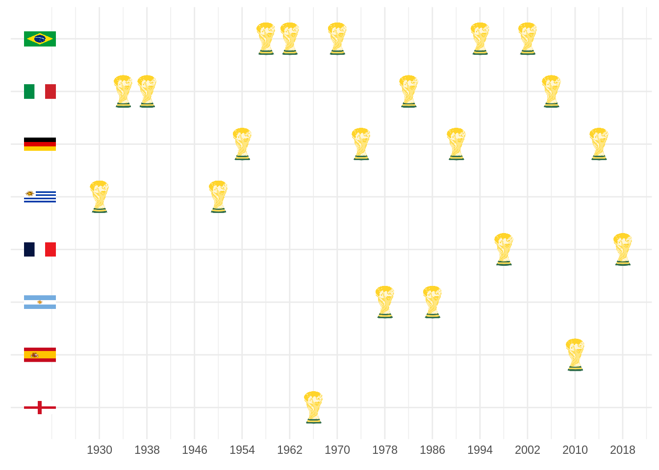
We observe here that Uruguay won its two World Cups in the first editions of the competition. We also see how Argentina, France and Spain have started to win World Cups recently.
With these two visualizations, I have presented some of the functionalities of ggplot2 to customize plots. I have also introduced ggimage package, that allows placing any image in plots done with ggplot2 with geom_image and geom_flag.
References
- FIFA World Cup dataset from Kaggle in tidytuesday repository: https://github.com/rfordatascience/tidytuesday/tree/master/data/2022/2022-11-29
- The first visualization was largely inspired by Paula’s blog R Functions and Packages for Political Science Analysis: https://rforpoliticalscience.com/2020/12/22/add-flags-to-graphs-with-ggimage-package-in-r/
- I have selected barplot colors inspired by this post compiled by R bloggers: https://www.r-bloggers.com/2012/05/bar-graph-colours-that-work-well/
Session info
## R version 4.2.2 Patched (2022-11-10 r83330)
## Platform: x86_64-pc-linux-gnu (64-bit)
## Running under: Linux Mint 19.2
##
## Matrix products: default
## BLAS:   /usr/lib/x86_64-linux-gnu/openblas/libblas.so.3
## LAPACK: /usr/lib/x86_64-linux-gnu/libopenblasp-r0.2.20.so
##
## locale:
##  [1] LC_CTYPE=es_ES.UTF-8       LC_NUMERIC=C
##  [3] LC_TIME=es_ES.UTF-8        LC_COLLATE=es_ES.UTF-8
##  [5] LC_MONETARY=es_ES.UTF-8    LC_MESSAGES=es_ES.UTF-8
##  [7] LC_PAPER=es_ES.UTF-8       LC_NAME=C
##  [9] LC_ADDRESS=C               LC_TELEPHONE=C
## [11] LC_MEASUREMENT=es_ES.UTF-8 LC_IDENTIFICATION=C
##
## attached base packages:
## [1] stats     graphics  grDevices utils     datasets  methods   base
##
## other attached packages:
##  [1] countrycode_1.4.0  tidytuesdayR_1.0.2 kableExtra_1.3.4   ggimage_0.3.1
##  [5] forcats_0.5.2      stringr_1.4.1      dplyr_1.0.10       purrr_0.3.5
##  [9] readr_2.1.3        tidyr_1.2.1        tibble_3.1.8       ggplot2_3.4.0
## [13] tidyverse_1.3.1
##
## loaded via a namespace (and not attached):
##  [1] httr_1.4.4         sass_0.4.1         jsonlite_1.8.3     viridisLite_0.4.1
##  [5] modelr_0.1.10      bslib_0.3.1        assertthat_0.2.1   highr_0.9
##  [9] yulab.utils_0.0.5  cellranger_1.1.0   yaml_2.3.6         pillar_1.8.1
## [13] backports_1.4.1    glue_1.6.2         digest_0.6.30      rvest_1.0.3
## [17] colorspace_2.0-3   ggfun_0.0.9        htmltools_0.5.3    pkgconfig_2.0.3
## [21] broom_1.0.1        haven_2.5.1        magick_2.7.3       bookdown_0.26
## [25] scales_1.2.1       webshot_0.5.3      ggplotify_0.1.0    svglite_2.1.0
## [29] tzdb_0.3.0         timechange_0.1.1   farver_2.1.1       generics_0.1.2
## [33] usethis_2.1.5      ellipsis_0.3.2     withr_2.5.0        cli_3.4.1
## [37] magrittr_2.0.3     crayon_1.5.2       readxl_1.4.1       evaluate_0.17
## [41] fs_1.5.2           fansi_1.0.3        xml2_1.3.3         blogdown_1.9
## [45] tools_4.2.2        hms_1.1.2          lifecycle_1.0.3    munsell_0.5.0
## [49] reprex_2.0.2       compiler_4.2.2     jquerylib_0.1.4    gridGraphics_0.5-1
## [53] systemfonts_1.0.4  rlang_1.0.6        grid_4.2.2         rstudioapi_0.13
## [57] labeling_0.4.2     rmarkdown_2.14     gtable_0.3.0       DBI_1.1.2
## [61] curl_4.3.2         R6_2.5.1           lubridate_1.9.0    knitr_1.40
## [65] fastmap_1.1.0      utf8_1.2.2         stringi_1.7.8      Rcpp_1.0.9
## [69] vctrs_0.5.0        dbplyr_2.2.1       tidyselect_1.1.2   xfun_0.34