In this post I will introduce how to perform analysis of variance (ANOVA) witb R. I will use dplyr and ggplot2 for data handling and visualization.
library(dplyr)
library(ggplot2)
Analysis of variance (ANOVA) is a statistical technique to examine if a treatment that splits the sample into \(t \geq 2\) categories affects a dependent variable \(y\), so that the average value of \(y\) for at least one of the treatments is different from the rest of treatments. ANOVA was created by Ronald Fisher in 1918 (Fisher, 1918). ANOVA is equivalent to examine the overall significance of the linear regression model:
\[ y_i = \beta_0 + \beta_1d_{1,i} + \dots + \beta_{t-1}d_{t_1,i} + \varepsilon_i\]
where \(d_j\) are binary or dummy variables equal to one if observation \(i\) has received treatment \(j\) and zero otherwise.
The approach of ANOVA is to decompose the variance of \(y\) into two terms: the variance explained by the treatment and the residual variance. We do that decomposing the sum of squares of \(y\) as follows:
\[ \sum_{i=1}^n \left(y_i - \bar{y}\right)^2 = \sum_{i=1}^n \left(\hat{y}_i - \bar{y}\right)^2 + \sum_{i=1}^n \left(y_i + \hat{y}_i\right)^2 \]
where \(\bar{y}\) is the mean of \(y\) for the whole sample and \(\hat{y}_i\) is the estimation of observation \(y_i\) by the linear regression model. This expression can be interpreted as that the total sum of squares \(TSS\) is equal to the sum of squares of the treatment \(SST\) plus the sum of squares of errors \(SSE\):
\[ TSS = SST + SSE\]
We can define terms analogous to variance for the treatment and the residuals dividing by their degrees of freedom. Then we obtain the mean of squares of treatment \(MST\) and the mean of squares of errors \(MSE\).
\[ \begin{align} MST &= \frac{SST}{t-1} & MSE &= \frac{SSE}{n-t} \end{align}\]
We examine if the treatment affects the dependent variable through an F-test. The null hypothesis of this tests can be stated as:
\[H_0: \mu_1 = \dots = \mu_p\]
If the null hypothesis holds, we have that:
\[ \frac{MST}{MSE} \sim F_{t-1, n-t} \]
where \(F_{t-1, n-t}\) is a F-Snedecor distribution with \(n_1= t-1\) and \(n_2 = n-t\). We can reject the null hypothesis if we obtain values of \(MST/MSE\) inusually large for a \(F_{t-1, n-t}\) distribution.
The validity assumptions of ANOVA are similar to the linear regression with ordinary least squares: observations must be independent and the residual variance \(MSE\) must follow a normal distribution with mean zero and equal variance across predicted values.
Applying ANOVA to the iris dataset
To perform an ANOVA analysis with R we need to:
- Define a linear model with the variable defining the category of each observation as independent variable, encoded as a factor.
- Run the
anovafunction with the defined linear model as argument.
Let’s do that with iris with Sepal.Length as dependent variable, and Species as categorical variable. As you may know, there are three different species of iris in the dataset: setosa, versicolor and virginica.
m1 <- lm(Sepal.Length ~ Species, data = iris)
anova(m1)
## Analysis of Variance Table
##
## Response: Sepal.Length
## Df Sum Sq Mean Sq F value Pr(>F)
## Species 2 63.212 31.606 119.26 < 2.2e-16 ***
## Residuals 147 38.956 0.265
## ---
## Signif. codes: 0 '***' 0.001 '**' 0.01 '*' 0.05 '.' 0.1 ' ' 1The outcome of the anova function is the ANOVA table:
- the treatment values are in the
Speciesrow, and the residuals inResiduals. - the column
Dfcontains the degrees of freedom,Sum Sqthe sums of squares andMean Sqeach sum of squares divided by its degrees of freedom. - columns
F valueandPr(>F)contain the results of the F-test.
The value of the F-test is an unlikely value for a F(2, 147) distribution. In fact, the 0.95 tail of this distribution is:
qf(0.95, 2, 172)## [1] 3.04852So it is safe to reject the null hypothesis here, and assert that the species an iris flower belongs to affects its sepal length.
Applying ANOVA with synthetic data
Let’s see what happens if population means of all treatments are equal. I have built a table with three different categories or treatments with 50 observations each. In all categories, the population mean of the dependent variable is equal to zero:
set.seed(1313)
df <- data.frame(y = rnorm(150), t = as.factor(c(rep("a", 50), rep("b", 50), rep("c", 50))))
df %>% glimpse()
## Rows: 150
## Columns: 2
## $ y <dbl> 1.18935584, 0.55138478, 0.35363427, -0.70397072, 0.11842555, -0.4236…
## $ t <fct> a, a, a, a, a, a, a, a, a, a, a, a, a, a, a, a, a, a, a, a, a, a, a,…Let’s see how the ANOVA looks like now:
mdf <- lm(y ~ t, df)
anova(mdf)
## Analysis of Variance Table
##
## Response: y
## Df Sum Sq Mean Sq F value Pr(>F)
## t 2 0.155 0.07764 0.0881 0.9157
## Residuals 147 129.602 0.88164In this case, the value of F is a plausible value of a F(2, 147) distribution, so we cannot reject the null hypothesis.
Let’s see what happens when we test ANOVA to a sample which means are equal in all categories but one. In df2 the mean of the dependent variable is 1 for category a, and zero for categories b and c.
df2 <- data.frame(y = c(rnorm(50, 1, 1), rnorm(100, 0, 1)), t = as.factor(c(rep("a", 50), rep("b", 50), rep("c", 50))))The results of ANOVA are:
mdf2 <- lm(y ~ t, df2)
anova(mdf2)
## Analysis of Variance Table
##
## Response: y
## Df Sum Sq Mean Sq F value Pr(>F)
## t 2 57.237 28.6184 26.879 1.125e-10 ***
## Residuals 147 156.511 1.0647
## ---
## Signif. codes: 0 '***' 0.001 '**' 0.01 '*' 0.05 '.' 0.1 ' ' 1The p-value is far lower than the usual benchmark of 0.05, so we can reject the null hypothesis. To see what’s going on with the means, we may plot confidence intervals for each of the mean:
ci <- \(t) mean_se(t, mult = 1.96)
ggplot(df2, aes(t, y)) +
  stat_summary(fun.data = ci) +
  labs(title = "95% CI for the mean for each treatment", x = "treatment", y = "dependent variable")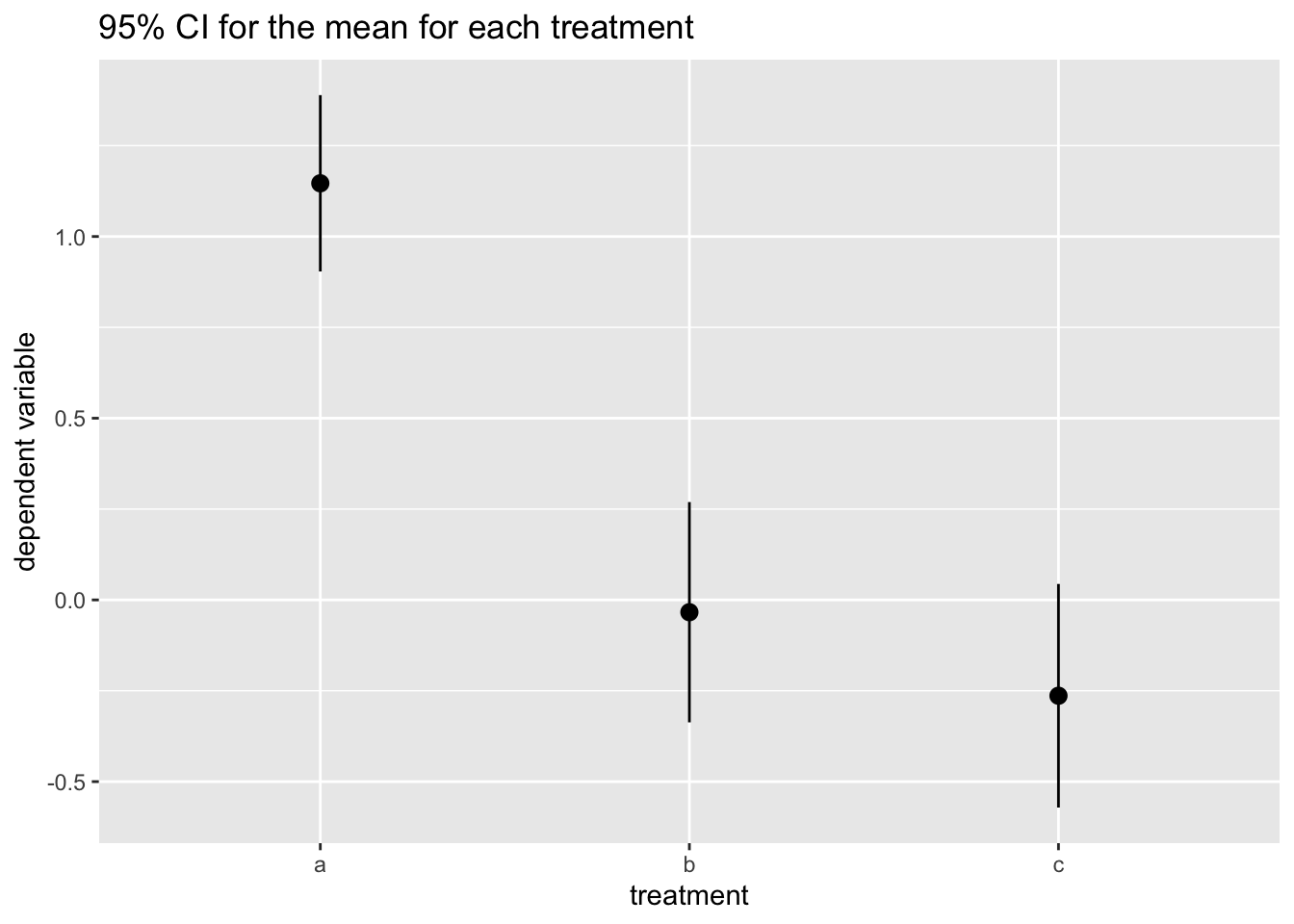
Here we observe that while confidence intervals for the mean overlap for b and c, the CI for category a does not overlap. This suggests that we cannot discard that population means for b and c are equal (or very close), while it is highly likely that category a has a higher mean.
Analysis of variance
Analysis of variance is a statistical technique for testing if the mean of a dependent variable is the same across the two or more categories the sample is divided. ANOVA splits total variance into two components: a component explained by the treatment and a residual component.
The null hypothesis of equality of the mean of the dependent variable across all categories can be tested with a F-test. If the mean of squares of the treatment is higher enough than the mean of squares of errors, we can discard the null hypothesis with a given confidence level.
The ANOVA in R is tested through a linear model that uses binary independent variables for each treatment, except the baseline. For the results of ANOVA to be valid, the sample should comply with the same requirements are ordinary least squares (OLS) regression. An ANOVA-like test of overall significance can be obtained for any OLS regression.
References
- Ronald Fisher (1918). The Correlation between Relatives on the Supposition of Mendelian Inheritance. Transactions of the Royal Society of Edinburgh, 52(2): 399-433.
Built with R 4.1.0, dplyr 1.0.7 and ggplot2 3.3.4