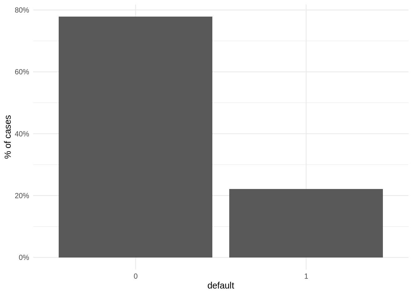
Setting workflow elements

Let’s define the elements of the tidymodels workflow. We start transforming the target default variable into a factor, setting the level of positive cases first.

LoanDefaults <- LoanDefaults %>%
  mutate(default = factor(default, levels = c("1", "0")))

Then, we need to split the data into train and test. As the dataset is large, I have selected a large prop value. Being the dataset unbalanced, it is important to set strata = default, so that the distribution of target variable in train and test sets will be similar to the original dataset. I have applied a similar logic to split the training set into four folds to apply cross validation.

set.seed(1313)
split <- initial_split(LoanDefaults, prop = 0.9, strata = "default")

folds <- vfold_cv(training(split), v = 10, strata = "default")

To evaluate model performance, I have chosen the following metrics:

• accuracy: fraction of observations correctly classified.
• sensitivity sens: the fraction of positive elements correctly classified.
• specificity spec: the fraction of negative elements correctly classified.
• area under the ROC curve roc_auc: a parameter assessing the tradeoff between sens and spec.

class_metrics <- metric_set(accuracy, sens, spec, roc_auc)

I will be using two models to train: a decision tree dt and a random forest rf. I will set standard values of parameter for each model. Hyperparameter tuning (not presented here) yields little influence of these parameters in model results.

dt <- decision_tree(mode = "classification", cost_complexity = 0.1, min_n = 10) %>%
  set_engine("rpart")

rf <- rand_forest(mode = "classification", trees = 50, mtry = 5, min_n = 10) %>%
  set_engine("ranger")

The preprocessing recipe is quite complex in this case:

• the variable ID is removed.
• variables PAY0 to PAY6 are removed. Before that, a payment_status variable is defined from PAY_0.
• variables payment_status, MARRIAGE and EDUCATION are transformed so that abormal values are set to NA.
• NA values of predictors are imputed usign k nearest neighbors.
• SEX, MARRIAGE and EDUCATION are transformed into factors.

rec_unb <- training(split) %>%
  recipe(default ~ .) %>%
  step_rm(ID) %>%
  step_mutate(payment_status = ifelse(PAY_0 < 1, 0, PAY_0)) %>%
  step_rm(PAY_0:PAY_6) %>%
  step_num2factor(SEX, levels = c("male", "female")) %>%
  step_mutate(MARRIAGE = ifelse(!MARRIAGE %in% 1:3, NA, MARRIAGE)) %>%
  step_mutate(EDUCATION = ifelse(!EDUCATION %in% 1:4, NA, EDUCATION)) %>%
  step_num2factor(MARRIAGE, levels = c("marriage", "single", "others")) %>% 
  step_num2factor(EDUCATION, levels = c("graduate", "university", "high_school", "others")) %>%
  step_impute_knn(all_predictors(), neighbors = 3)

Now we can test the two models using cross validation. We start with the decision tree:

dt_cv_unb <- fit_resamples(object = dt,
                       preprocessor = rec_unb,
                       resamples = folds,
                       metrics = class_metrics)

rf_cv_unb <- fit_resamples(object = rf,
                       preprocessor = rec_unb,
                       resamples = folds,
                       metrics = class_metrics)

The metrics for the decision tree are:

dt_cv_unb %>%
  collect_metrics()

## # A tibble: 4 × 6
##   .metric  .estimator  mean     n  std_err .config             
##   <chr>    <chr>      <dbl> <int>    <dbl> <chr>               
## 1 accuracy binary     0.820    10 0.00140  Preprocessor1_Model1
## 2 roc_auc  binary     0.644    10 0.00321  Preprocessor1_Model1
## 3 sens     binary     0.329    10 0.00661  Preprocessor1_Model1
## 4 spec     binary     0.959    10 0.000712 Preprocessor1_Model1

And the metrics for cross validation:

rf_cv_unb %>%
  collect_metrics()

## # A tibble: 4 × 6
##   .metric  .estimator  mean     n std_err .config             
##   <chr>    <chr>      <dbl> <int>   <dbl> <chr>               
## 1 accuracy binary     0.818    10 0.00242 Preprocessor1_Model1
## 2 roc_auc  binary     0.759    10 0.00374 Preprocessor1_Model1
## 3 sens     binary     0.360    10 0.00680 Preprocessor1_Model1
## 4 spec     binary     0.948    10 0.00176 Preprocessor1_Model1

The sensitivity of the two models is quite low. This is not good, because it means that a default will be undetected using these models.

Model with undersampling

A commonly used technique to improve classification of unbalanced data is to modify the training set so that it has the same number of positives and negatives. There are two ways of doing this:

• oversampling: creating additional artificial observations for the less frequent case.
• undersampling: removing observations of the most frequent case.

In tidymodels, those recipes are implemented with the themis package.

For this dataset, I have decided to undersample the training set using the step_downsample. The use of oversampling has lead to unsatisfactory results.

rec_us <- rec_unb %>%
  step_downsample(default, under_ratio = 1)

Let’s examine the distribution of the target variable after downsampling:

rec_us %>%
  prep() %>%
  juice() %>%
    ggplot(aes(factor(default))) + 
  geom_bar(aes(y = (..count..)/sum(..count..))) +
  scale_y_continuous(labels=percent) +
  labs(x = "default", y = "% of cases") +
  theme_minimal()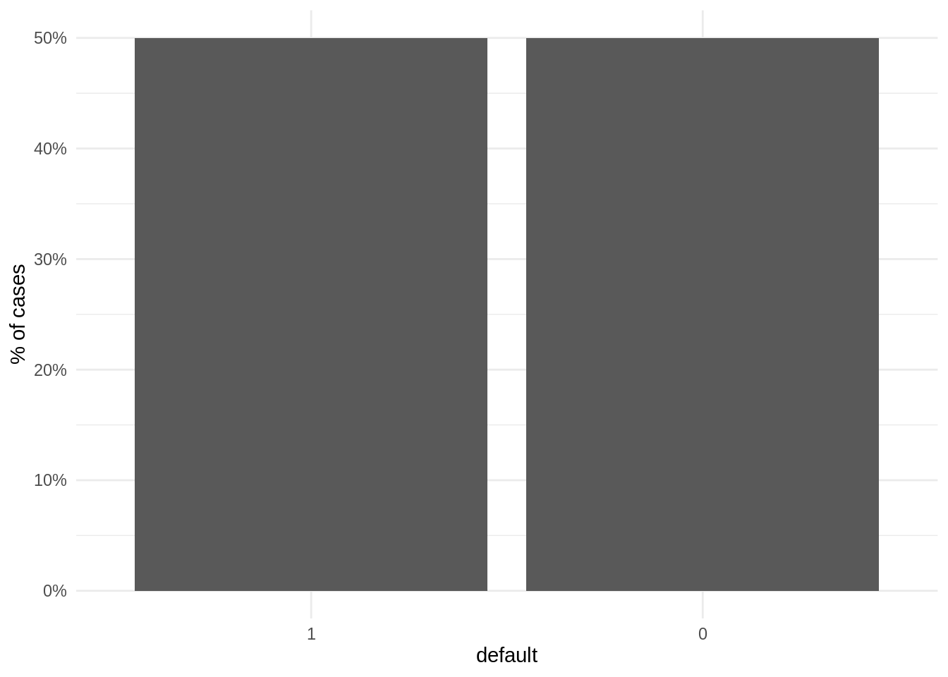

We observe that all the dataset for which is trained the model is balanced. Let’s proceed to train the models with the undersampled recipe:

dt_cv_us <- fit_resamples(object = dt,
                       preprocessor = rec_us,
                       resamples = folds,
                       metrics = class_metrics)

rf_cv_us <- fit_resamples(object = rf,
                       preprocessor = rec_us,
                       resamples = folds,
                       metrics = class_metrics)

As the metrics are presented in data frames, we can put them all together and examine the performance of the four models at once. As variability of metrics can be an issue when balancing data, I have added errorbars for each parameter.

t1 <- dt_cv_unb %>%
  collect_metrics() %>%
  mutate(model = "tree", train = "unbalanced")

t2 <- rf_cv_unb %>%
  collect_metrics() %>%
  mutate(model = "forest", train = "unbalanced")

t3 <- dt_cv_us %>%
  collect_metrics() %>%
  mutate(model = "tree", train = "balanced")

t4 <- rf_cv_us %>%
  collect_metrics() %>%
  mutate(model = "forest", train = "balanced")

bind_rows(t1, t2, t3, t4) %>%
  ggplot(aes(x =.metric, y = mean, ymin = mean - std_err, ymax = mean + std_err, fill = train)) +
  geom_bar(stat = "identity", position = "dodge") +
  geom_errorbar(position=position_dodge(width=1), width = 0.5) +
  scale_fill_manual(values = c("#990000", "#FF8000")) +
  facet_grid(. ~ model) +
  labs(x = "metric", y = "value")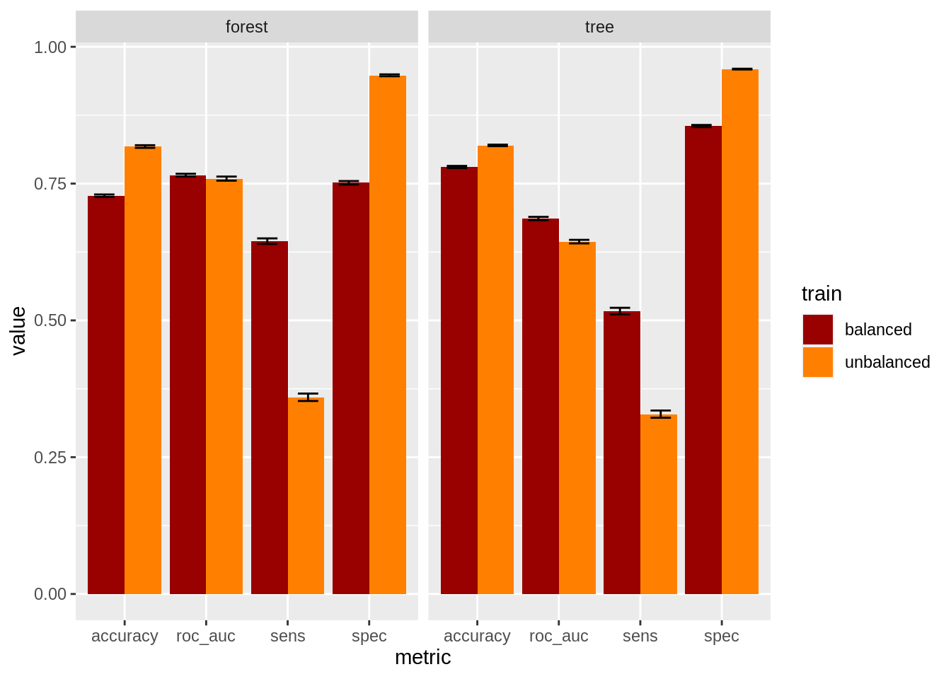

We can observe that undersampling increases values of sensitivity at the cost of reducing specificity. Undersampling leads to slightly worse values of accuracy, and slightly better values of AUC.

Prediction for the undersampled model

Let’s choose the undersampled model trained with the random forest model. We can test this model on both the test and train set.

We start defining the model using a workflow:

rf_us <- workflow() %>%
  add_recipe(rec_us) %>%
  add_model(rf) %>%
  fit(training(split))

Let’s obtain the predicted values for train and test sets. Note that the prediction on the train set is with the original data, not with the undersampled ones. Undersampling only takes place to fit the model.

pred_train <- rf_us %>%
  predict(training(split)) %>%
  bind_cols(training(split) %>% select(default))

pred_test <- rf_us %>%
  predict(testing(split)) %>%
  bind_cols(testing(split) %>% select(default))

The confusion matrices show that the model tends to inflate false positives to obtain a decent value of specifity:

class_metrics2 <- metric_set(accuracy, sens, spec)

pred_train %>%
  conf_mat(truth = default, estimate = .pred_class)

##           Truth
## Prediction     1     0
##          1  5870  3941
##          0   102 17086

pred_test %>%
  conf_mat(truth = default, estimate = .pred_class)

##           Truth
## Prediction    1    0
##          1  430  572
##          0  234 1765

Let’s compare accuracy, sensitivity and specificity for train and test sets:

class_metrics2 <- metric_set(accuracy, sens, spec)

t_train <- pred_train %>%
  class_metrics2(truth = default, estimate = .pred_class) %>%
  mutate(set = "train")
t_test <- pred_test %>%
  class_metrics2(truth = default, estimate = .pred_class) %>% 
  mutate(set = "test")

bind_rows(t_train, t_test) %>%
  ggplot(aes(.metric, .estimate, fill = set)) +
  geom_bar(stat = "identity", position = "dodge") +
  scale_fill_manual(values = c("#990000", "#FF8000")) +
  labs(x = "metric", y = "value") +
  theme_minimal()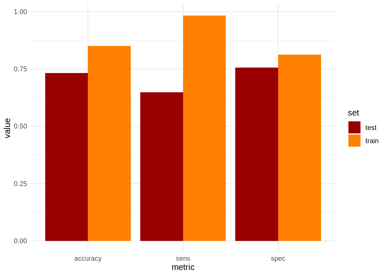

We observe that undersampling has improved sensitivity at the price of worsening accuracy and specificity. In this case, undersampling has somewhat improved our model, but this is not always the case. Specially when we use oversampling, where we introduce artificial observations to train the model. Some alternative approaches to deal with unbalanced datasets can be found at the StackExchange question cited below.

References

• BAdatasets page: https://github.com/jmsallan/BAdatasets
• themis package website: https://themis.tidymodels.org/
• StackExchange question: Are unbalanced datasets problematic, and (how) does oversampling (purport to) help? https://stats.stackexchange.com/questions/357466/are-unbalanced-datasets-problematic-and-how-does-oversampling-purport-to-he
• Yeh, I. C., & Lien, C. H. (2009). The comparisons of data mining techniques for the predictive accuracy of probability of default of credit card clients. Expert Systems with Applications, 36(2), 2473-2480. https://doi.org/10.1016/j.eswa.2007.12.020

Session info

sessionInfo()

## R version 4.2.1 (2022-06-23)
## Platform: x86_64-pc-linux-gnu (64-bit)
## Running under: Linux Mint 19.2
## 
## Matrix products: default
## BLAS:   /usr/lib/x86_64-linux-gnu/openblas/libblas.so.3
## LAPACK: /usr/lib/x86_64-linux-gnu/libopenblasp-r0.2.20.so
## 
## locale:
##  [1] LC_CTYPE=es_ES.UTF-8       LC_NUMERIC=C              
##  [3] LC_TIME=es_ES.UTF-8        LC_COLLATE=es_ES.UTF-8    
##  [5] LC_MONETARY=es_ES.UTF-8    LC_MESSAGES=es_ES.UTF-8   
##  [7] LC_PAPER=es_ES.UTF-8       LC_NAME=C                 
##  [9] LC_ADDRESS=C               LC_TELEPHONE=C            
## [11] LC_MEASUREMENT=es_ES.UTF-8 LC_IDENTIFICATION=C       
## 
## attached base packages:
## [1] stats     graphics  grDevices utils     datasets  methods   base     
## 
## other attached packages:
##  [1] ranger_0.13.1      rpart_4.1.16       BAdatasets_0.1.0   themis_0.2.1      
##  [5] yardstick_0.0.9    workflowsets_0.2.1 workflows_0.2.6    tune_0.2.0        
##  [9] tidyr_1.2.0        tibble_3.1.6       rsample_0.1.1      recipes_0.2.0     
## [13] purrr_0.3.4        parsnip_0.2.1      modeldata_0.1.1    infer_1.0.0       
## [17] ggplot2_3.3.5      dplyr_1.0.9        dials_0.1.1        scales_1.2.0      
## [21] broom_0.8.0        tidymodels_0.2.0  
## 
## loaded via a namespace (and not attached):
##  [1] lubridate_1.8.0    doParallel_1.0.17  DiceDesign_1.9     tools_4.2.1       
##  [5] backports_1.4.1    bslib_0.3.1        utf8_1.2.2         R6_2.5.1          
##  [9] DBI_1.1.2          colorspace_2.0-3   nnet_7.3-17        withr_2.5.0       
## [13] tidyselect_1.1.2   parallelMap_1.5.1  compiler_4.2.1     cli_3.3.0         
## [17] labeling_0.4.2     bookdown_0.26      sass_0.4.1         checkmate_2.1.0   
## [21] stringr_1.4.0      digest_0.6.29      rmarkdown_2.14     unbalanced_2.0    
## [25] pkgconfig_2.0.3    htmltools_0.5.2    parallelly_1.31.1  lhs_1.1.5         
## [29] highr_0.9          fastmap_1.1.0      rlang_1.0.2        rstudioapi_0.13   
## [33] BBmisc_1.12        FNN_1.1.3          farver_2.1.0       jquerylib_0.1.4   
## [37] generics_0.1.2     jsonlite_1.8.0     magrittr_2.0.3     ROSE_0.0-4        
## [41] Matrix_1.5-1       Rcpp_1.0.8.3       munsell_0.5.0      fansi_1.0.3       
## [45] GPfit_1.0-8        lifecycle_1.0.1    furrr_0.3.0        stringi_1.7.6     
## [49] pROC_1.18.0        yaml_2.3.5         MASS_7.3-58        plyr_1.8.7        
## [53] grid_4.2.1         parallel_4.2.1     listenv_0.8.0      crayon_1.5.1      
## [57] lattice_0.20-45    splines_4.2.1      mlr_2.19.0         knitr_1.39        
## [61] pillar_1.7.0       future.apply_1.9.0 codetools_0.2-18   fastmatch_1.1-3   
## [65] glue_1.6.2         evaluate_0.15      ParamHelpers_1.14  blogdown_1.9      
## [69] data.table_1.14.2  vctrs_0.4.1        foreach_1.5.2      RANN_2.6.1        
## [73] gtable_0.3.0       future_1.25.0      assertthat_0.2.1   xfun_0.30         
## [77] gower_1.0.0        prodlim_2019.11.13 class_7.3-20       survival_3.4-0    
## [81] timeDate_3043.102  iterators_1.0.14   hardhat_0.2.0      lava_1.6.10       
## [85] globals_0.14.0     ellipsis_0.3.2     ipred_0.9-12