In this post, I will present how oversampling and undersampling can help us in a classification job on an unbalanced dataset. In unbalanced datasets, the target variable has an uneven distribution, with salient majority and minority classes. Undersampling and oversampling try to improve model performance training the model with a balanced dataset. When using undersampling, we train the model with a set removing observations of the majority class. With oversampling, we train the model with a dataset with additional artificial elements of the minority class.
I will be using tidymodels for the prediction workflow, BAdatasets to access the dataset and themis to perform undersampling and oversampling.
library(tidymodels)
library(themis)
library(BAdatasets)
I will be using the cc_defaults dataset. It is a dataset of defaults payments in Taiwan, presented in Yeh & Lien (2009).
data("cc_defaults")When plotting the proportion of observations for each case, we observe that the number of negative cases (not defaulted) is much larger than the positive cases (defaulted). Therefore, the set of positive cases is the minority class. This is a frequent situation in contexts like loan defaults or credit card fraud.
cc_defaults |>
  ggplot(aes(factor(default))) +
  geom_bar(aes(y = after_stat(count)/sum(after_stat(count)))) +
  scale_y_continuous(labels=percent) +
  labs(x = "default", y = "% of cases") +
  theme_minimal()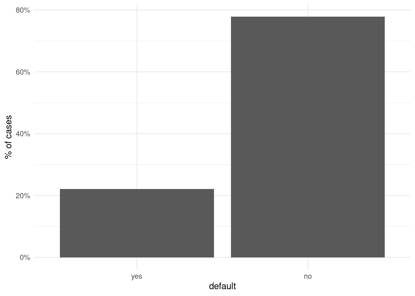
Workflow elements
Let’s define the elements of the tidymodels workflow. We start transforming the target default variable into a factor, setting the level of positive cases first.
cc_defaults <- cc_defaults |>
  mutate(default = factor(default, levels = c("yes", "no")))
Then, we need to split the data into train and test. As the dataset is large, I have selected a large prop value to include in the train set. Being the dataset unbalanced, it is important to set strata = "default", so that the distribution of target variable in train and test sets will be similar to the original dataset. I have applied a similar logic to split the training set into five folds to apply cross validation.
set.seed(1313)
split <- initial_split(cc_defaults, prop = 0.9, strata = "default")

folds <- vfold_cv(training(split), v = 5, strata = "default")
To evaluate model performance, I have chosen the following metrics:
accuracy: fraction of observations correctly classified.- sensitivity
sens: the fraction of positive elements correctly classified. - specificity
spec: the fraction of negative elements correctly classified. - area under the ROC curve
roc_auc: a parameter assessing the tradeoff betweensensandspec.
class_metrics <- metric_set(accuracy, sens, spec, roc_auc)In unbalanced datasets, accuracy can be a bad metric of performance. If 90% of observations belong to the negative class, we obtain an accuracy of 0.9 simply classifying all observations as negative. In that context, usually sensitivity is a more adequate metric. Additionally, in jobs like loan defaults or credit card fraud, the cost of a false negative is much higher than of a false positive.
I will use a decision tree dt model, setting standard parameters.
dt <- decision_tree(mode = "classification", cost_complexity = 0.1, min_n = 10) |>
  set_engine("rpart")
The preprocessing recipe has the following steps:
- variables
idandpay_septopay_aprare removed. Before that, I am replacingpay_sepwith payment_status. - variables
payment_status,marriageandeducationare transformed so that abnormal values are set toNA. NAvalues of predictors are imputed usign k nearest neighbors.
rec_base <- training(split) |>
  recipe(default ~ .) |>
  step_rm(id) |>
  step_mutate(payment_status = ifelse(pay_sep < 1, 0, pay_sep)) |>
  step_rm(pay_sep:pay_apr) |>
  step_mutate(marriage = ifelse(!marriage %in% 1:3, NA, marriage)) |>
  step_mutate(education = ifelse(!education %in% 1:4, NA, education)) |>
  step_impute_knn(impute_with = all_predictors(), neighbors = 5)
The steps to perform undersampling and oversampling are provided by themis package. Here I am using the following methods:
step_downsampleperforms random majority under-sampling with replacement.step_upsampleperforms random minority over-sampling with replacement.
These steps are added to the rec_base recipe to obtain new recipes rec_us and rec_os for under and oversampling, respectively.
rec_us <- rec_base |>
  step_downsample(default, under_ratio = 1)

rec_os <- rec_base |>
  step_upsample(default, over_ratio = 1)
Testing under- and oversampling with cross validation
Now we are ready to test each of the three models with cross validation. ´cv_unb,cv_usandcv_os` train the model with the original dataset, undersampling and oversampling respectively.
cv_unb <- fit_resamples(object = dt,
                        preprocessor = rec_base,
                        resamples = folds,
                        metrics = class_metrics)

cv_us <- fit_resamples(object = dt,
                        preprocessor = rec_us,
                        resamples = folds,
                        metrics = class_metrics)

cv_os <- fit_resamples(object = dt,
                        preprocessor = rec_os,
                        resamples = folds,
                        metrics = class_metrics)
Now we can extract the metrics for each of the cross-validations. We can stack them all in a single data frame m.
m_unb <- collect_metrics(cv_unb) |>
  mutate(train = "unbalanced")

m_us <- collect_metrics(cv_us) |>
  mutate(train = "undersampling")

m_os <- collect_metrics(cv_os) |>
  mutate(train = "oversampling")

m <- bind_rows(m_unb, m_us, m_os) |>
  mutate(train = factor(train, levels = c("unbalanced", "undersampling", "oversampling")))
Let’s see the results:
ggplot(m, aes(.metric, mean, fill = train)) +
  geom_bar(stat = "identity", position = "dodge") +
  theme_minimal() +
  labs(title = "Performance of cross validation", x = "metric", y = "value")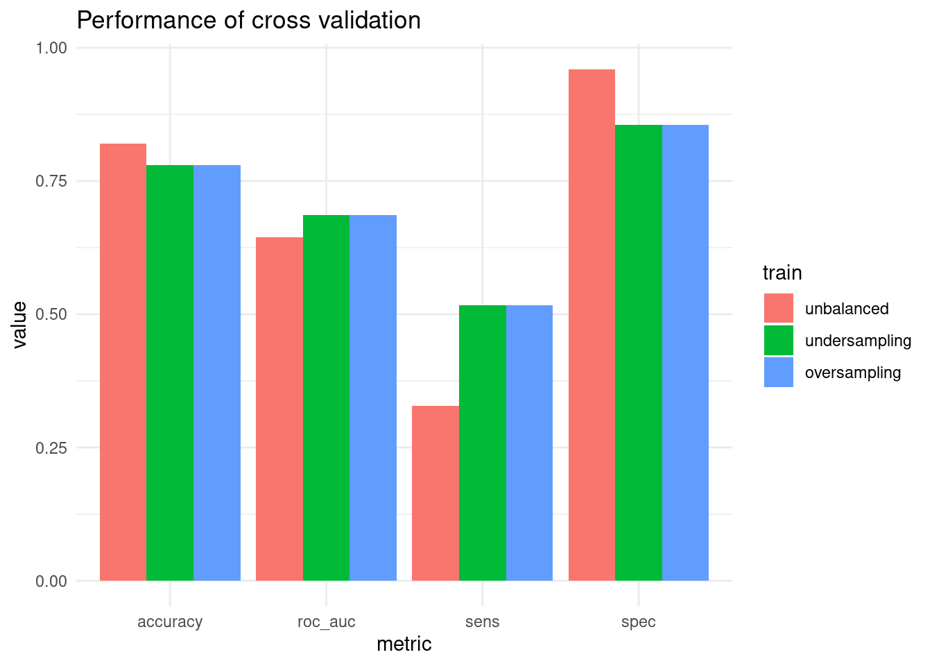
In this case, oversampling and undersampling obtain the same results. Both allow improving sensitivity significantly (although the obtained value is quite poor), paying the price of slightly worsening specificity. Global parameters like accuracy and AUC are not significantly affected.
Evaluating the model in the test set
Now I will fit the model with the whole train set and examine its performance in the test set. In class_metrics2 I am excluding roc_auc because I will obtain the class predicted only.
class_metrics2 <- metric_set(accuracy, sens, spec)Objects unb_model, us_model and os_model contain the model trained in the original, undersampled and oversampled recipes respectively.
unb_model <- workflow() |>
  add_recipe(rec_base) |>
  add_model(dt) |>
  fit(training(split))

us_model <- workflow() |>
  add_recipe(rec_us) |>
  add_model(dt) |>
  fit(training(split))

os_model <- workflow() |>
  add_recipe(rec_os) |>
  add_model(dt) |>
  fit(training(split))
Next, I am storing in df_test the results of evaluating each of the models in the test set. Note that we evaluate the model in the original dataset. Under- and oversampling are only performed to train the model. The datasets where the model is evaluated are not modified.
m_test <- lapply(list(unb_model, us_model, os_model), function(x) x |>
         predict(testing(split)) |>
         bind_cols(testing(split)) |>
         class_metrics2(truth = default, estimate = .pred_class))
df_test <- bind_rows(m_test) |>
  mutate(train = rep(c("unbalanced", "undersampling", "oversampling"), each = 3)) |>
  mutate(train = factor(train, levels = c("unbalanced", "undersampling", "oversampling")))
Here are the results of the evaluation. They are quite similar to the obtained with cross validation.
ggplot(df_test, aes(.metric, .estimate, fill = train)) +
  geom_bar(stat = "identity", position = "dodge") +
  theme_minimal() +
  labs(title = "Performance of test set", x = "metric", y = "value")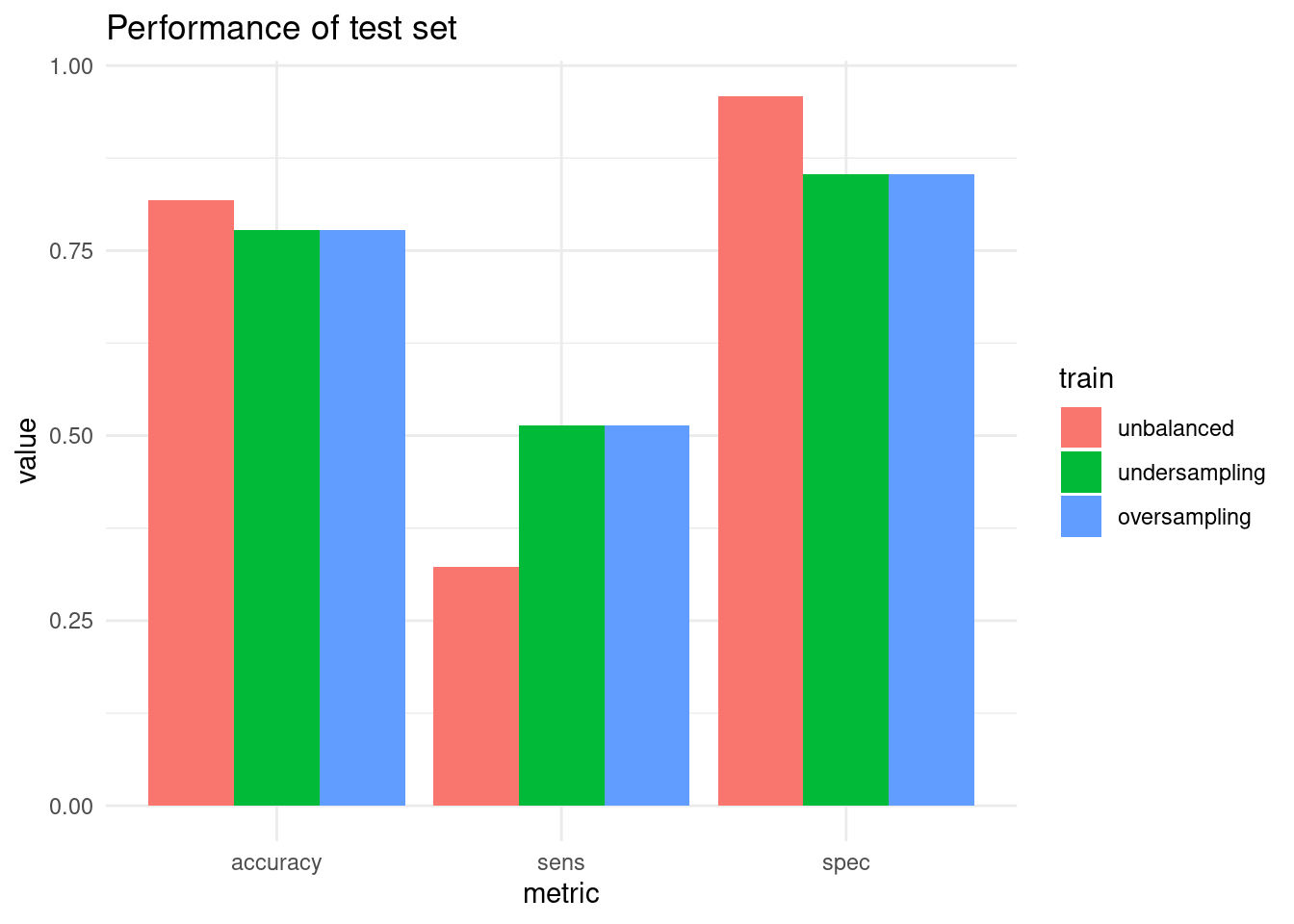
Under- and oversampling can be useful techniques to improve the ratio of true evaluations of the minority class in unbalanced datasets. So these techniques tend to increase sensitivity at the price of worse values of specificity. This can be a good compromise in classification jobs where the cost of a false positive is much higher than of a false negative.
References
BAdatasetspackage https://github.com/jmsallan/BAdatasetsthemispackage website: https://themis.tidymodels.org/- Yeh, I. C., & Lien, C. H. (2009). The comparisons of data mining techniques for the predictive accuracy of probability of default of credit card clients. Expert Systems with Applications, 36(2), 2473-2480. https://doi.org/10.1016/j.eswa.2007.12.020
Session info
## R version 4.4.2 (2024-10-31)
## Platform: x86_64-pc-linux-gnu
## Running under: Linux Mint 21.1
##
## Matrix products: default
## BLAS:   /usr/lib/x86_64-linux-gnu/blas/libblas.so.3.10.0
## LAPACK: /usr/lib/x86_64-linux-gnu/lapack/liblapack.so.3.10.0
##
## locale:
##  [1] LC_CTYPE=es_ES.UTF-8       LC_NUMERIC=C
##  [3] LC_TIME=es_ES.UTF-8        LC_COLLATE=es_ES.UTF-8
##  [5] LC_MONETARY=es_ES.UTF-8    LC_MESSAGES=es_ES.UTF-8
##  [7] LC_PAPER=es_ES.UTF-8       LC_NAME=C
##  [9] LC_ADDRESS=C               LC_TELEPHONE=C
## [11] LC_MEASUREMENT=es_ES.UTF-8 LC_IDENTIFICATION=C
##
## time zone: Europe/Madrid
## tzcode source: system (glibc)
##
## attached base packages:
## [1] stats     graphics  grDevices utils     datasets  methods   base
##
## other attached packages:
##  [1] rpart_4.1.23       BAdatasets_0.2.0   themis_1.0.2       yardstick_1.3.1
##  [5] workflowsets_1.1.0 workflows_1.1.4    tune_1.2.1         tidyr_1.3.1
##  [9] tibble_3.2.1       rsample_1.2.1      recipes_1.0.10     purrr_1.0.2
## [13] parsnip_1.2.1      modeldata_1.3.0    infer_1.0.7        ggplot2_3.5.1
## [17] dplyr_1.1.4        dials_1.2.1        scales_1.3.0       broom_1.0.5
## [21] tidymodels_1.2.0
##
## loaded via a namespace (and not attached):
##  [1] tidyselect_1.2.1    timeDate_4032.109   farver_2.1.1
##  [4] fastmap_1.1.1       blogdown_1.19       digest_0.6.35
##  [7] timechange_0.3.0    lifecycle_1.0.4     ellipsis_0.3.2
## [10] survival_3.8-3      magrittr_2.0.3      compiler_4.4.2
## [13] rlang_1.1.3         sass_0.4.9          tools_4.4.2
## [16] utf8_1.2.4          yaml_2.3.8          data.table_1.15.4
## [19] knitr_1.46          labeling_0.4.3      DiceDesign_1.10
## [22] withr_3.0.0         nnet_7.3-20         grid_4.4.2
## [25] fansi_1.0.6         colorspace_2.1-0    future_1.33.2
## [28] globals_0.16.3      iterators_1.0.14    MASS_7.3-64
## [31] cli_3.6.2           rmarkdown_2.26      generics_0.1.3
## [34] rstudioapi_0.16.0   future.apply_1.11.2 cachem_1.0.8
## [37] splines_4.4.2       parallel_4.4.2      vctrs_0.6.5
## [40] hardhat_1.3.1       Matrix_1.7-1        jsonlite_1.8.8
## [43] bookdown_0.39       listenv_0.9.1       foreach_1.5.2
## [46] gower_1.0.1         jquerylib_0.1.4     glue_1.7.0
## [49] parallelly_1.37.1   codetools_0.2-19    lubridate_1.9.3
## [52] gtable_0.3.5        munsell_0.5.1       GPfit_1.0-8
## [55] ROSE_0.0-4          pillar_1.9.0        furrr_0.3.1
## [58] htmltools_0.5.8.1   ipred_0.9-14        lava_1.8.0
## [61] R6_2.5.1            lhs_1.2.0           evaluate_0.23
## [64] lattice_0.22-5      highr_0.10          backports_1.4.1
## [67] bslib_0.7.0         class_7.3-23        Rcpp_1.0.12
## [70] prodlim_2023.08.28  xfun_0.43           pkgconfig_2.0.3
Modified for small typos and dataset update on 2025-01-13.