In this post, I will present how to use the ggraph and tidygraph packages to represent large networks. I will take air transport data from the OpenFlights dataset stored in the BAdatasetsSpatial package to present the airport networks of two airlines following different business models: Ryanair and KLM.
library(BAdatasetsSpatial)
library(dplyr)
library(ggplot2)
library(tidygraph)
library(ggraph)
The Ryanair network
The of_routes data frame contains routes stored in the OpenFlights database. Those data are of historic interest, as they were collected around June 2014.
head(of_routes)## airline org dst codeshare stops equipment
## 1 2B AER KZN N 0 CR2
## 2 2B ASF KZN N 0 CR2
## 3 2B ASF MRV N 0 CR2
## 4 2B CEK KZN N 0 CR2
## 5 2B CEK OVB N 0 CR2
## 6 2B DME KZN N 0 CR2Let’s start with Ryanair, an airline following the low-cost carrier business model. Airlines following this business model do not offer connecting flights and scheduled their routes on a point-to-point network. We start selecting the Ryanair flights:
ryanair_table <- of_routes %>%
  filter(airline == "FR") %>%
  select(org, dst)
And then using the tbl_graph function of tidygraph to construct a tbl_graph - igraph object. Data on nodes and edges is stored in two different tables:
ryanair <- tbl_graph(edge = ryanair_table, directed = TRUE)
ryanair
## # A tbl_graph: 176 nodes and 2484 edges
## #
## # A directed simple graph with 1 component
## #
## # Node Data: 176 × 1 (active)
## name
## <chr>
## 1 AAR
## 2 AGP
## 3 PMI
## 4 STN
## 5 ACE
## 6 BCN
## # … with 170 more rows
## #
## # Edge Data: 2,484 × 2
## from to
## <int> <int>
## 1 1 2
## 2 1 3
## 3 1 4
## # … with 2,481 more rowsWe reach the node data table using activate to compute two measures of node centrality: degree and betweenness. Nodes with high values of these measures are considered central nodes in the network. To allow comparison between network, I am normalizing these measures using the graph_order function, that returns the number of nodes of the graph. As the graph is directed, I am considering degree the sum of in- and out-degree.
ryanair <- ryanair %>%
  activate(nodes) %>%
  mutate(deg = (centrality_degree(mode = "in") + centrality_degree(mode = "out"))/(2*(graph_order() - 1)),
         btw = centrality_betweenness()/((graph_order() - 1)*(graph_order() - 2)))
Here I am using the as_tibble() function to get the node table and present the airports of highest degree:
ryanair %>%
  activate(nodes) %>%
  as_tibble() %>%
  arrange(-deg)
## # A tibble: 176 × 3
## name deg btw
## <chr> <dbl> <dbl>
## 1 STN 0.709 0.365
## 2 DUB 0.434 0.0802
## 3 CRL 0.429 0.106
## 4 BGY 0.36 0.0404
## 5 AGP 0.286 0.0301
## 6 PMI 0.28 0.0277
## 7 BVA 0.263 0.0190
## 8 CIA 0.257 0.0113
## 9 GRO 0.251 0.0323
## 10 HHN 0.246 0.0244
## # … with 166 more rowsAnd the airports of highest betweenness:
ryanair %>%
  activate(nodes) %>%
  as_tibble() %>%
  arrange(-btw)
## # A tibble: 176 × 3
## name deg btw
## <chr> <dbl> <dbl>
## 1 STN 0.709 0.365
## 2 CRL 0.429 0.106
## 3 DUB 0.434 0.0802
## 4 OPO 0.206 0.0457
## 5 MRS 0.194 0.0440
## 6 BGY 0.36 0.0404
## 7 BCN 0.223 0.0365
## 8 GRO 0.251 0.0323
## 9 AGP 0.286 0.0301
## 10 PMI 0.28 0.0277
## # … with 166 more rowsWe can even plot degree against betweenness straight from the tbl_graph object:
ryanair_nodes <- ryanair %>%
  activate(nodes) %>%
  as_tibble()

ggplot(ryanair_nodes, aes(deg, btw)) +
  geom_point() +
  geom_text(data = ryanair_nodes %>% filter(deg > 0.3), aes(label = name), nudge_y = 0.015) +
  labs(title = "Degree vs. betwenness (Ryanair)", x = "degree", y = "betweenness") +
  theme_minimal()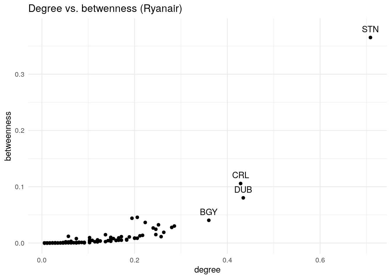
The most central airports of this Ryanair network are London-Stansted (STN), Dubin (DUB),Brussels South Charleroi (CRL) and Oriol al Serio (BGY).
Let’s use ggraph to plot the Ryanair network with ggraph. The default plot is not very encouraging:
set.seed(1313)
ryanair %>%
  ggraph +
  geom_edge_link() +
  geom_node_point() +
  geom_node_text(aes(label = name))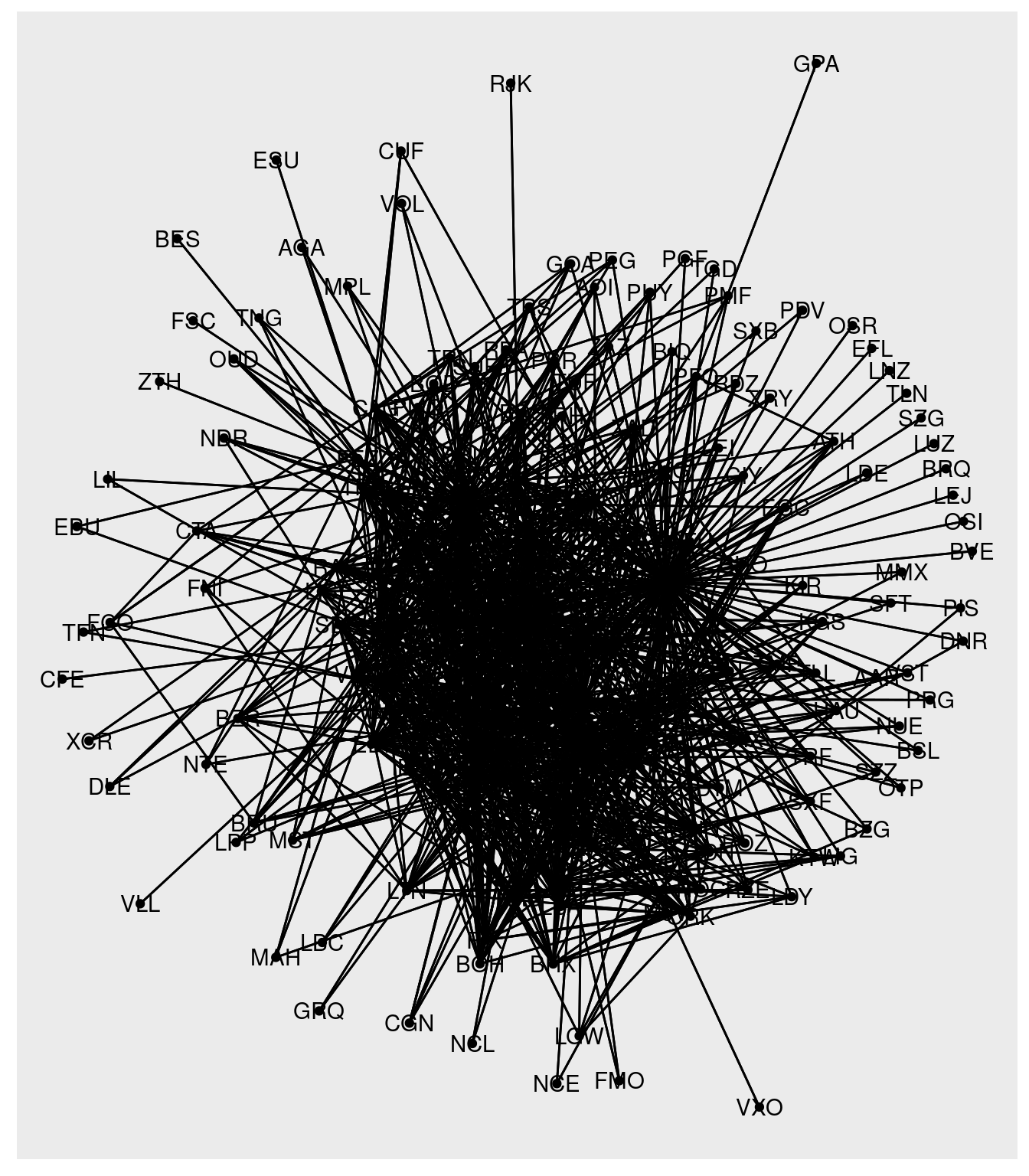
Here I have done some tuning of the output to plot a nicer graph:
- I have chosen
kkamong the several layouts available fromigraph. You can see them here or typing?layout_tbl_graph_igraphin the console. - To make visible node labels, it is a good idea to make edges transparent. Here I have used a very low value of
alphaingeom_edge_link. - The color of nodes is proportional to its betweenness. The scale of colors has been tuned with
scale_color_gradient. sizeandnudgeof text labels has been tuned up through trial and error.- I have used the
theme_graph()and I have removed the legend intheme.
set.seed(1313)
ryanair %>%
  ggraph(layout = 'kk') +
  geom_edge_link(alpha = 0.05) +
  geom_node_point(aes(colour = btw), size = 2) +
  geom_node_text(aes(label = name), size = 2, nudge_x = 0.3) +
  scale_color_gradient(low = "#CCFFFF", high = "#006666") +
  theme_graph() +
  theme(legend.position = "none")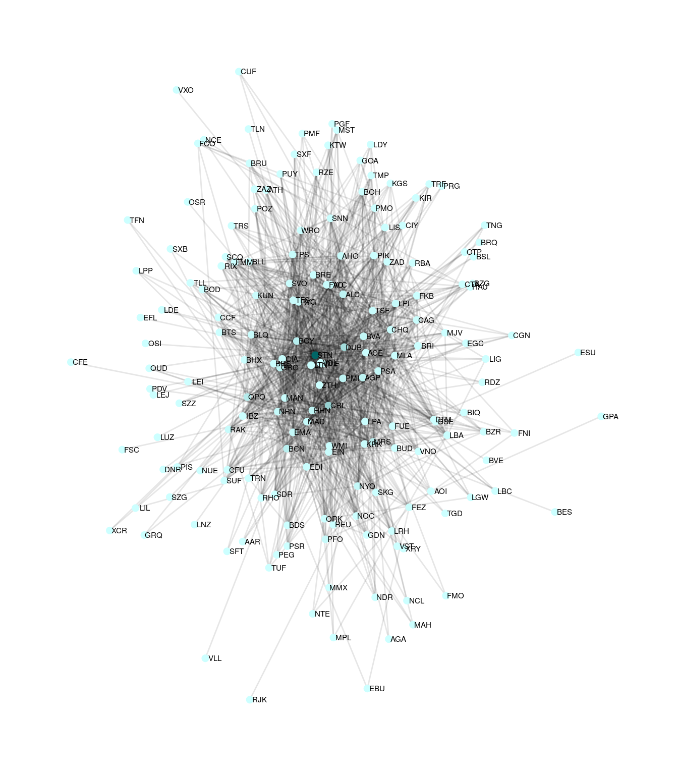
The resulting network is typical of a point-to-point network. Each flight is operated independently, and no connecting flights are offered by the airline.
The KLM network of operated flights
Let’s examine now the KLM network. KLM follows the full-service carrier business model, so it has a hub-and-spoke network. I start defining the klm network object:
klm_table <- of_routes %>%
  filter(airline == "KL") %>%
  select(org, dst, codeshare)

klm <- tbl_graph(edge = klm_table, directed = TRUE)
We see now that edges have a codeshare attribute: edges with value N are operated by KLM, and edges with Y are marketed by KLM through codeshare agreements, but operated by other companies. This is a a common practice among full-service carriers.
klm## # A tbl_graph: 368 nodes and 830 edges
## #
## # A directed simple graph with 1 component
## #
## # Node Data: 368 × 1 (active)
## name
## <chr>
## 1 AAL
## 2 AMS
## 3 ABE
## 4 ATL
## 5 ABQ
## 6 ABV
## # … with 362 more rows
## #
## # Edge Data: 830 × 3
## from to codeshare
## <int> <int> <chr>
## 1 1 2 Y
## 2 3 4 Y
## 3 5 4 Y
## # … with 827 more rowsLet’s define the network klm_own of routes operated by KLM. I have removed the nodes not included in this network by removing the nodes with degree equal to zero:
klm_own <- klm %>%
    activate(edges) %>%
  filter(codeshare == "N") %>%
  activate(nodes) %>%
  mutate(deg = centrality_degree()) %>%
  filter(deg !=0) %>%
  select(-deg)
Now I am computing the normalized measures of degree and betweenness:
klm_own <- klm_own %>%
  activate(nodes) %>%
  mutate(deg = (centrality_degree(mode = "in") + centrality_degree(mode = "out"))/(2*(graph_order() - 1)),
         btw = centrality_betweenness()/((graph_order() - 1)*(graph_order() - 2)))
We observe that the Amsterdam-Schipol airport (AMS) has the highest values of degree and betweenness. These values are close to one for this airport, suggesting an almost star network centered in AMS.
klm_own %>%
  activate(nodes) %>%
  as_tibble() %>%
  arrange(-btw)
## # A tibble: 107 × 3
## name deg btw
## <chr> <dbl> <dbl>
## 1 AMS 0.892 0.998
## 2 AUH 0.0189 0.0189
## 3 DOH 0.0189 0.0189
## 4 EZE 0.0189 0.0189
## 5 KUL 0.0189 0.0189
## 6 SIN 0.0189 0.0189
## 7 TPE 0.0189 0.0189
## 8 AUA 0.00943 0.00943
## 9 CUR 0.0142 0.00943
## 10 HRE 0.00943 0.00943
## # … with 97 more rowsThis intuition is confirmed by when we plot the network. This airport network is a hub-and spoke network, where connections between airports are secured through connecting flights at the hub:
set.seed(1313)
klm_own %>%
  ggraph(layout = "fr") +
  geom_edge_link(alpha = 0.05) +
  geom_node_point(size = 2) +
  geom_node_text(aes(label = name), size = 2, nudge_x = 0.4) +
  theme_graph()
The KLM network of operated flights
Let’s examine now the network of flights marketed (operated or not) by KLM:
klm <- klm %>%
  activate(nodes) %>%
  mutate(deg = (centrality_degree(mode = "in") + centrality_degree(mode = "out"))/(2*(graph_order() - 1)),
         btw = centrality_betweenness()/((graph_order() - 1)*(graph_order() - 2)))
The degree-betwenness plot presents two highly central nodes: Amsterdam-Schipol and Hartsfield–Jackson Atlanta International Airport (ATL). ATL is the hub of Delta Airlines. Delta and KLM are both members of the SkyTeam airline alliance.
klm_nodes <- klm %>%
  activate(nodes) %>%
  as_tibble()

ggplot(klm_nodes, aes(deg, btw)) +
  geom_point() +
  geom_text(data = klm_nodes %>% filter(deg > 0.2), aes(label = name), nudge_y = 0.02) +
  labs(title = "Degree vs. betwenness (KLM)", x = "degree", y = "betweenness") +
  theme_minimal()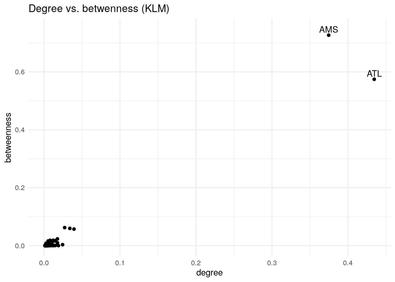
Here is the network of flights marketed by KLM. I have used the same tricks as Ryanair, adding now a color to edges depending if they correspond to flights operated (op) or marketed only (mk) by KLM. We can see how KLM extends its airport network to the United States thorugh its partnership with Delta Airlines and its participation in the SkyTeam alliance.
set.seed(1313)
klm %>%
  ggraph(layout = "kk") +
  geom_edge_link(aes(color = codeshare), alpha = 0.1) +
  geom_node_point(size = 1) +
  geom_node_text(aes(label = name), size = 2, nudge_x = 0.4) +
  scale_edge_color_manual(name = "flight", labels = c("op", "mk"), values = c("#0000FF", "#FF0000")) +
  theme_graph()  +
  theme(legend.position = "bottom")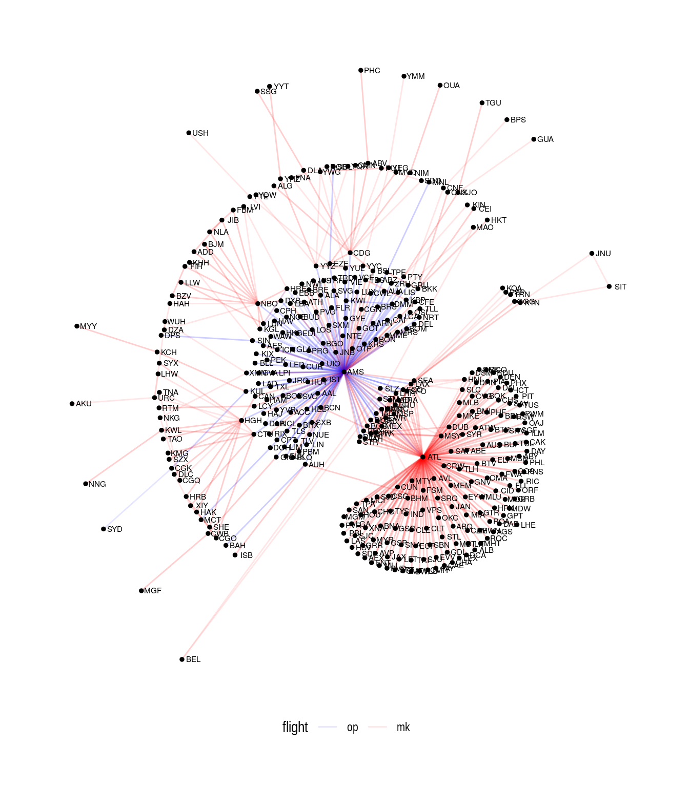
References
- Hoffman, M. (2021). Centrality, in Methods for Network Analysis. https://bookdown.org/markhoff/social_network_analysis/centrality.html (reference on degree, betweenness and other centrality measures).
- OpenFlights (2014). Airport, airline and route data https://openflights.org/data.html
- Pedersen, T. L. (2017). Introducing tidygraph. https://www.data-imaginist.com/2017/introducing-tidygraph/
- Pedersen, T. L. (2017). Introduction to ggraph: nodes. https://www.data-imaginist.com/2017/ggraph-introduction-nodes/
- Pedersen, T. L. (2017). Introduction to ggraph: edges. https://www.data-imaginist.com/2017/ggraph-introduction-edges/
- Pedersen, T. L. (2017). Introduction to ggraph: layouts. https://www.data-imaginist.com/2017/ggraph-introduction-layouts/
- Sallan, J. M. (2021).
BAdatasetsSpatialR package. https://github.com/jmsallan/BAdatasetsSpatial - Sallan, J. M. & Lordan, O. (2019). Air Route Networks Through Complex Networks Theory. Elsevier. https://doi.org/10.1016/C2016-0-02288-X (see chapter 2 for a more detailed discussion on airline business models).
Session info
## R version 4.1.2 (2021-11-01)
## Platform: x86_64-pc-linux-gnu (64-bit)
## Running under: Debian GNU/Linux 10 (buster)
##
## Matrix products: default
## BLAS:   /usr/lib/x86_64-linux-gnu/blas/libblas.so.3.8.0
## LAPACK: /usr/lib/x86_64-linux-gnu/lapack/liblapack.so.3.8.0
##
## locale:
##  [1] LC_CTYPE=es_ES.UTF-8       LC_NUMERIC=C
##  [3] LC_TIME=es_ES.UTF-8        LC_COLLATE=es_ES.UTF-8
##  [5] LC_MONETARY=es_ES.UTF-8    LC_MESSAGES=es_ES.UTF-8
##  [7] LC_PAPER=es_ES.UTF-8       LC_NAME=C
##  [9] LC_ADDRESS=C               LC_TELEPHONE=C
## [11] LC_MEASUREMENT=es_ES.UTF-8 LC_IDENTIFICATION=C
##
## attached base packages:
## [1] stats     graphics  grDevices utils     datasets  methods   base
##
## other attached packages:
## [1] ggraph_2.0.5            tidygraph_1.2.0         ggplot2_3.3.5
## [4] dplyr_1.0.7             BAdatasetsSpatial_0.1.0 sf_1.0-2
##
## loaded via a namespace (and not attached):
##  [1] tidyselect_1.1.1   xfun_0.23          bslib_0.2.5.1      graphlayouts_0.7.2
##  [5] purrr_0.3.4        colorspace_2.0-1   vctrs_0.3.8        generics_0.1.0
##  [9] viridisLite_0.4.0  htmltools_0.5.1.1  yaml_2.2.1         utf8_1.2.1
## [13] rlang_0.4.12       e1071_1.7-8        jquerylib_0.1.4    pillar_1.6.4
## [17] glue_1.4.2         withr_2.4.2        DBI_1.1.1          tweenr_1.0.2
## [21] lifecycle_1.0.0    stringr_1.4.0      munsell_0.5.0      blogdown_1.5
## [25] gtable_0.3.0       evaluate_0.14      labeling_0.4.2     knitr_1.33
## [29] class_7.3-19       fansi_0.5.0        highr_0.9          Rcpp_1.0.6
## [33] KernSmooth_2.23-20 scales_1.1.1       classInt_0.4-3     jsonlite_1.7.2
## [37] farver_2.1.0       gridExtra_2.3      ggforce_0.3.3      digest_0.6.27
## [41] stringi_1.7.3      ggrepel_0.9.1      bookdown_0.24      polyclip_1.10-0
## [45] grid_4.1.2         cli_3.0.1          tools_4.1.2        magrittr_2.0.1
## [49] sass_0.4.0         proxy_0.4-26       tibble_3.1.5       crayon_1.4.1
## [53] tidyr_1.1.4        pkgconfig_2.0.3    ellipsis_0.3.2     MASS_7.3-54
## [57] rstudioapi_0.13    viridis_0.6.1      assertthat_0.2.1   rmarkdown_2.9
## [61] R6_2.5.0           units_0.7-2        igraph_1.2.6       compiler_4.1.2