Triangular and PERT probability distributions are used to model uncertainty in situations, like project management, where we have limited information about the variable we are modelling. In the context of project management, these are frequently used to model the duration of activities. Both distributions model variables based on three parameters:
- Minimum value \(a\).
- Most likely value \(m\), or mode (not to be confused with the mean or average value).
- Maximum value \(b\).
In this post, I will introduce how to use the mc2d package to model triangular and PERT distributions. I will also use the tidyverse for data handling and plotting.
library(tidyverse)
library(mc2d)
The Triangular Distribution
The distribution function of a triangular distribution consists of straight lines connecting the three parameters of the distribution, scaled to obtain a triangle of area equal to one. Let’s see an example with values 5,000, 7,000 and 11,000. I will use seq() to obtain 1,000 values evenly spaced between maximum and minimum.
values <- seq(5000, 11000, length.out = 1000)Let’s see how the triangular probability density distribution looks like, using the mc2d::dtriang() function.
td <- tibble(values = values,
             shape = "triangular",
             dist = dtriang(values, min = 5000, mode = 7000, max = 11000))

ggplot(td, aes(values, dist)) +
  geom_line(linewidth = 1) +
  theme_minimal() +
  scale_x_continuous(breaks = seq(5000, 11000, 2000), limits = c(4500, 11500)) +
  labs(x = NULL, y = NULL, title = "The Triangular Distribution")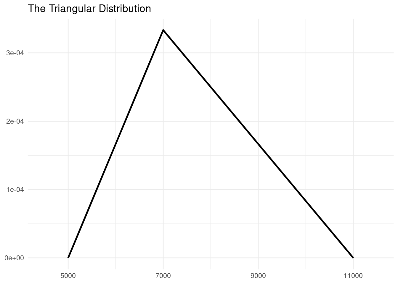
The PERT Distribution
PERT stands for Program Evaluation and Review Technique, a technique used for project management where the use of probability distributions is quite frequent. THe PERT distribution comes from the beta distribution, and it is modelled so that has minimum \(a\) and maximum \(c\) with mean equal to:
\[ \mu = \frac{a + 4m + b}{6} \]
We can use the mc2d::dpert() function to obtain the PERT probability density function.
pd <- tibble(values = values,
             shape = "PERT",
             dist = dpert(values, min = 5000, mode = 7000, max = 11000))

ggplot(pd, aes(values, dist)) +
  geom_line(linewidth = 1) +
  theme_minimal() +
  scale_x_continuous(breaks = seq(5000, 11000, 2000), limits = c(4500, 11500)) +
  labs(x = NULL, y = NULL, title = "The PERT Distribution")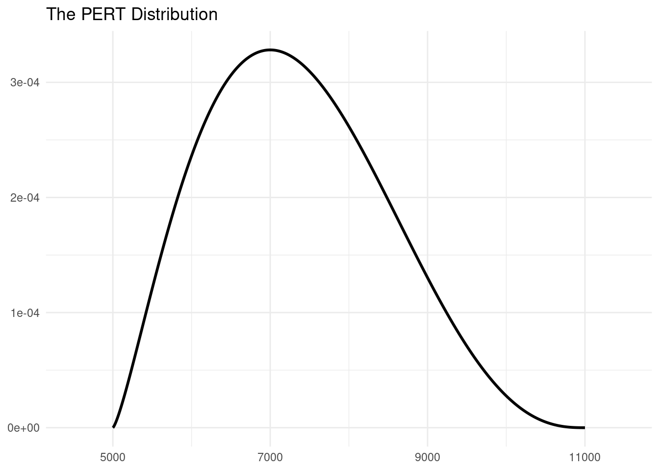
Let’s compare the two probability density distributions to appreciate its differences.
ad <- bind_rows(td, pd)

ggplot(ad, aes(values, dist, color = shape)) +
  geom_line(linewidth = 1) +
  theme_minimal() +
  scale_x_continuous(breaks = seq(5000, 11000, 2000), limits = c(4500, 11500)) +
  labs(x = NULL, y = NULL, title = "Triangular and PERT Distribution") +
  scale_color_manual(name = "Distribution", values = c("#FF0000", "#0000FF")) +
  theme(legend.position = "bottom")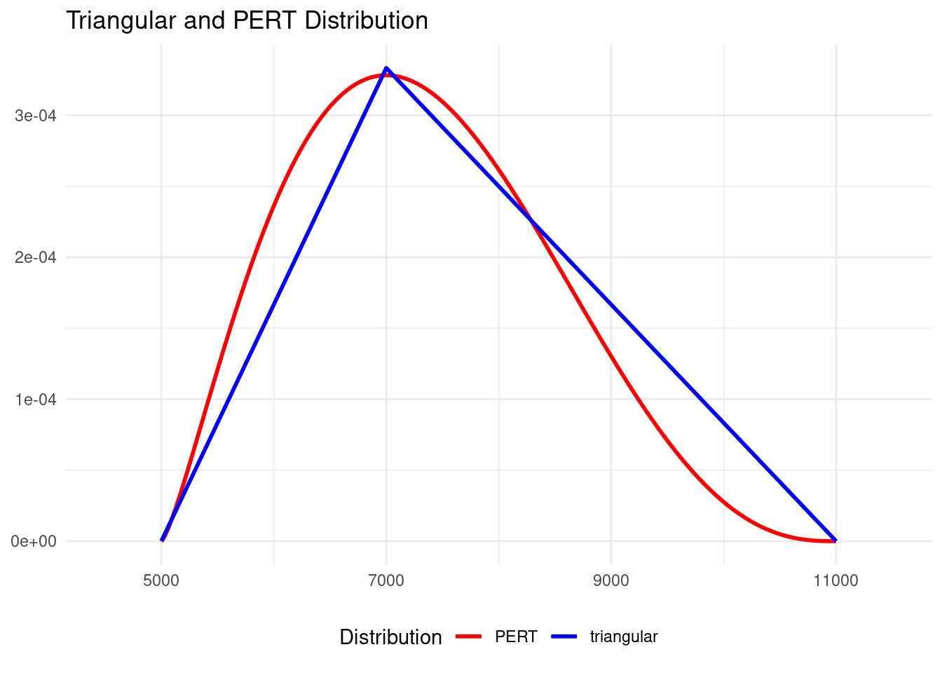
Compared with the triangular distribution, the PERT distribution is scaled up so that the probability of the mode \(m\) is roughly similar for both distributions, while values around the bound furthest from the mode have lower probabilities. In the above plot, as \(m\) is closer to \(a\) than to \(b\), values of duration closer to the upper bound have a low probability of occurrence.
Shape of PERT Distribution
A more generic family of PERT distributions can be obtained depending upon a \(\gamma\) shape parameter so that the mean is equal to:
\[ \mu = \frac{a + \gamma m + b}{\gamma + 2} \]
Note that the PERT distribution presented above has \(\gamma = 4\). It is the PERT distribution closer to the triangular distribution, so it is taken as the default value.
To examine the impact of this parameter in the probability density function we can make:
pert_values <- map_dfr(2:6, ~ tibble(values = values,
                      shape = .,
                      dist = dpert(values, min = 5000, mode = 7000, max = 11000, shape = ., log = FALSE))) |>
  mutate(shape = as.character(shape))

pert_values |>
  ggplot(aes(values, dist, color = shape)) +
  geom_line() +
  scale_color_manual(values = c("#FF6666", "#CC0000", "black", "#0000CC", "#6666FF")) +
  scale_x_continuous(breaks = seq(5000, 11000, 2000),
                     limits = c(4500, 11500)) +
  theme_minimal() +
  theme(legend.position = "bottom") +
  labs(x = NULL, y = NULL, title = "Values of Shape of PERT Distribution")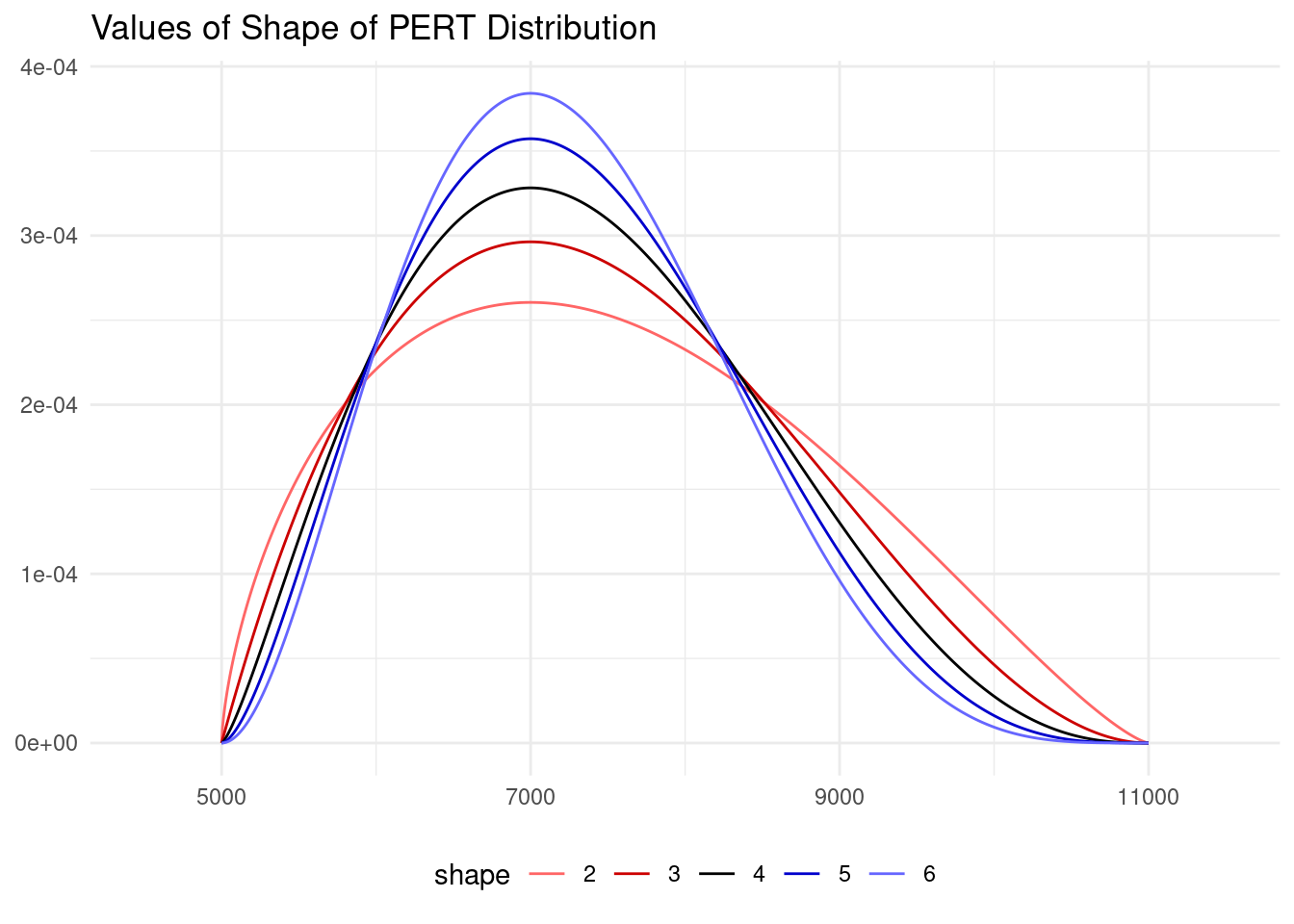
Values of the shape parameter higher than four will lead to distributions more centered around the mode, so that extreme values will have a lower probability of occurrence.
Triangular and PERT Distributions
Triangular and PERT probability distributions are used to model uncertainty in situations where we have information about the maximum, minimum and more frequent values of a variable. These distributions have been used extensively in project management, specially when using Monte Carlo simulations to model projects with uncertain duration.
Session Info
## R version 4.4.1 (2024-06-14)
## Platform: x86_64-pc-linux-gnu
## Running under: Linux Mint 21.1
##
## Matrix products: default
## BLAS:   /usr/lib/x86_64-linux-gnu/blas/libblas.so.3.10.0
## LAPACK: /usr/lib/x86_64-linux-gnu/lapack/liblapack.so.3.10.0
##
## locale:
##  [1] LC_CTYPE=es_ES.UTF-8       LC_NUMERIC=C
##  [3] LC_TIME=es_ES.UTF-8        LC_COLLATE=es_ES.UTF-8
##  [5] LC_MONETARY=es_ES.UTF-8    LC_MESSAGES=es_ES.UTF-8
##  [7] LC_PAPER=es_ES.UTF-8       LC_NAME=C
##  [9] LC_ADDRESS=C               LC_TELEPHONE=C
## [11] LC_MEASUREMENT=es_ES.UTF-8 LC_IDENTIFICATION=C
##
## time zone: Europe/Madrid
## tzcode source: system (glibc)
##
## attached base packages:
## [1] stats     graphics  grDevices utils     datasets  methods   base
##
## other attached packages:
##  [1] mc2d_0.2.1      mvtnorm_1.2-5   lubridate_1.9.3 forcats_1.0.0
##  [5] stringr_1.5.1   dplyr_1.1.4     purrr_1.0.2     readr_2.1.5
##  [9] tidyr_1.3.1     tibble_3.2.1    ggplot2_3.5.1   tidyverse_2.0.0
##
## loaded via a namespace (and not attached):
##  [1] sass_0.4.9        utf8_1.2.4        generics_0.1.3    rstatix_0.7.2
##  [5] blogdown_1.19     stringi_1.8.3     hms_1.1.3         digest_0.6.35
##  [9] magrittr_2.0.3    evaluate_0.23     grid_4.4.1        timechange_0.3.0
## [13] bookdown_0.39     fastmap_1.1.1     jsonlite_1.8.8    backports_1.4.1
## [17] fansi_1.0.6       scales_1.3.0      jquerylib_0.1.4   abind_1.4-5
## [21] cli_3.6.2         rlang_1.1.3       munsell_0.5.1     withr_3.0.0
## [25] cachem_1.0.8      yaml_2.3.8        tools_4.4.1       tzdb_0.4.0
## [29] ggsignif_0.6.4    colorspace_2.1-0  ggpubr_0.6.0      broom_1.0.5
## [33] vctrs_0.6.5       R6_2.5.1          lifecycle_1.0.4   car_3.1-2
## [37] pkgconfig_2.0.3   pillar_1.9.0      bslib_0.7.0       gtable_0.3.5
## [41] glue_1.7.0        highr_0.10        xfun_0.43         tidyselect_1.2.1
## [45] rstudioapi_0.16.0 knitr_1.46        farver_2.1.1      htmltools_0.5.8.1
## [49] labeling_0.4.3    carData_3.0-5     rmarkdown_2.26    compiler_4.4.1