In the tidymodels framework, a prediction job usually consists of a preprocessing recipe and the application of a model to the preprocessed data set. The use of recipes allows applying the preprocessing to any test data to be assessed, using parameters of the train set to avoid data leaking.
A particularly hard problem to tackle are unbalanced classification problems, where the levels of the target variable appear with different probabilities. In problems like credit card fraud prediction or attrition prediction, it is critical to predict correctly the less like level of the target variable (i.e., the existence of fraud or employee attrition). As models tend to overestimate the probability of the majority class, some specific steps must be taken to foster model quality. A frequent strategy (no the only one) to achieve this is to train models with a balanced dataset. This is achieved either by oversampling (adding artificial data of the minority class) or by undersampling (removing a fraction of the data of the majority class). In tidymodels, this is done with the pre-processing steps delivered by the themis package.
The recipe and the model are put together with functions of the workflows package. If we are using more than one combination of preprocessing and model, it can be useful to test them at once. We can do that with the functionalities of the workflowsets package.
The performance of a specific model may depend on specific parameters that cannot be learned from the training set, called hyperparameters. In tidymodels, hyperparameter tuning is performed with the tune:tune_grid() function. This process can be guided through functions of the dials package, such as dials:grid_regular().
In this post, I will present a tidymodels workflow to predict employee attrition with the attrition dataset from modeldata. The workflow test the combination of three pre-processing recipes and a logistic regression model using the glmnet package that implements regularized regression. The recipes include oversampling and undersampling, and the best version of the regularized regression model is obtained through hyperparameter tuning. Then, we are using workflow sets and a regular tuning grid scheme.
Let’s start loading the packages we need and the dataset.
library(tidymodels)
library(themis)

data("attrition")
I will set the positive case as first level of the target variable to get the right values of sensitivity and specificity.
attrition <- attrition |>
  mutate(Attrition = factor(Attrition, levels = c("Yes", "No")))
Doing a barplot we confirm that the dataset is unbalanced.
attrition |>
  ggplot(aes(Attrition)) +
  geom_bar()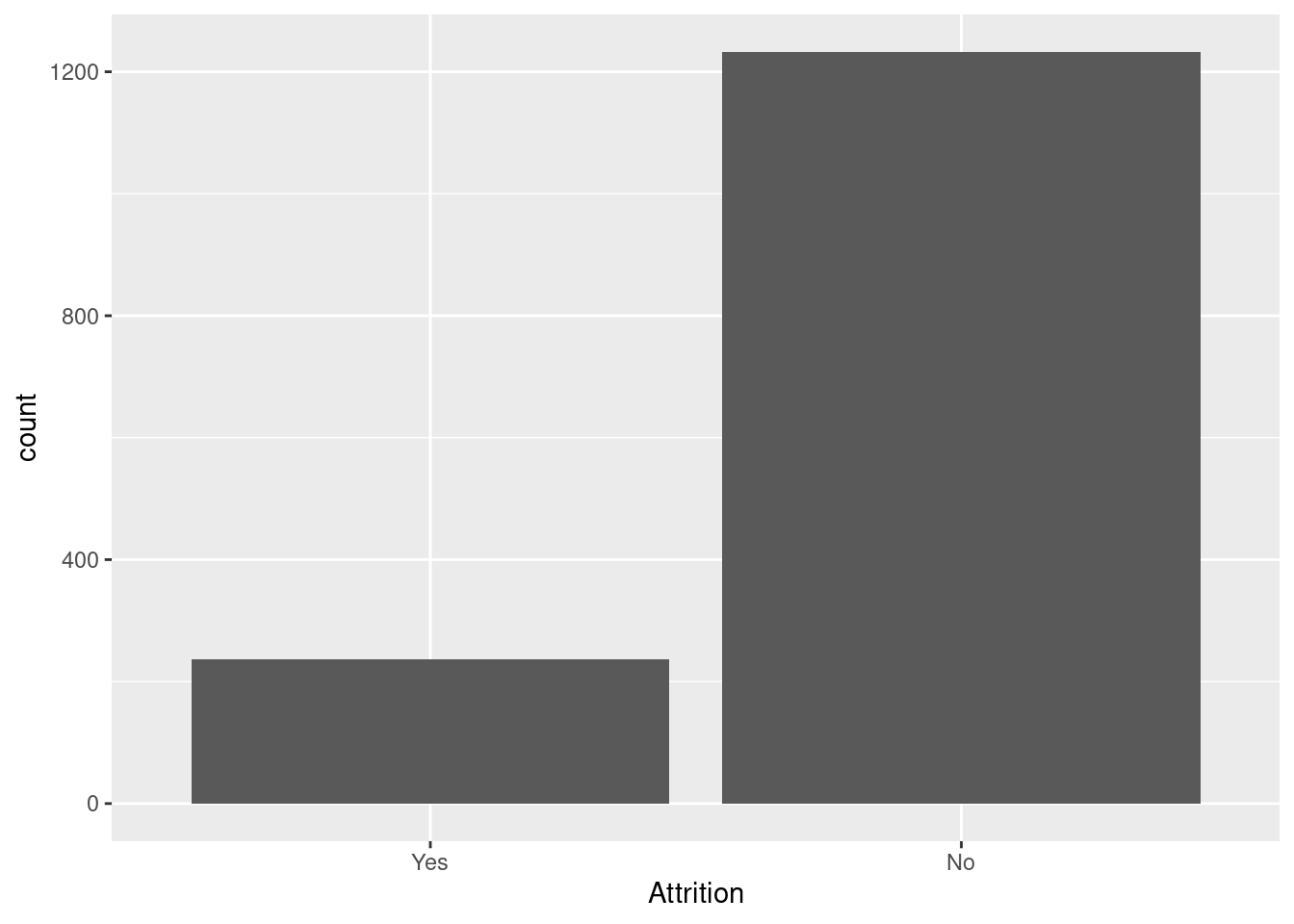
As the dataset is relatively small, I am assigning a 85% to train and 15% to test. Samples are obtained with stratification of the target variable.
set.seed(11)
at_split <- initial_split(attrition, prop = 0.85, strata = "Attrition")
Pre-processing
I am setting three pre-processing recipes:
- A baseline recipe
at_rec. It includes thestep_nzv()andstep_corr()filters. Oversampling schemes and theglmnetfunctions work with numerical variables only, so I include a step_dummy() step to transform each nominal predictor into a set of dummy variables. - An undersampling recipe
at_downsample, obtained by addingstep_downsample()to the baseline. - An oversampling recipe
at_oversample, adding nowstep_smote().
at_rec <- recipe(Attrition ~ ., training(at_split)) |>
  step_nzv(all_predictors()) |>
  step_corr(all_numeric_predictors()) |>
  step_dummy(all_nominal_predictors())

at_downsample <- at_rec |>
  step_downsample(Attrition, under_ratio = 1)

at_oversample <- at_rec |>
  step_smote(Attrition, over_ratio = 1)
The model
The dataset has many variables, and adding all of them can result in a noisy model. Regularized regression tackles that automating feature selection by adding penalty terms to the squared sum of regressions. In lasso (L1) regression the term is equal to the sum of absolute values of coefficients and in ridge regression (L2) is equal to the sum of squared coefficients. While L1 regression tends to set some coefficients to zero, L2 tends to reduce coefficient values for noisy variables. Both terms can be combined in a model, so we have elastic nets.
In parsnip, logistic_reg() with glmmet has two tuning parameters:
- the amount of regularization
penalty. - the proportion of lasso penalty
mixture, somixture = 1means L1 regression,mixture = 0L2 regression and intermediate values elastic nets. In thelrmodel, we set the values to be tuned withtune().
lr <- logistic_reg(mode = "classification",
                   engine = "glmnet",
                   penalty = tune(),
                   mixture = tune())
The functions of the grid package provide typical values for tuning parameters. lr_grid is a regular grid of 5 levels of each parameter, so there are 25 combinations of tuning parameters to be tested.
lr_grid <- grid_regular(penalty(),
                        mixture(),
                        levels = 5)
Folds and Metrics
To test each combination of tuning parameters for a workflow, I am defining a cross validation scheme with six folds of the training set. These are also stratified by the target variable.
set.seed(44)
folds <- vfold_cv(training(at_split), v= 6, strata = "Attrition")
To assess performance, I addition to accuracy, sensitivity and specifity I am using the J-index, equal to sensitivity plus specificity minus one. I will obtained these metrics with a tailored class_metrics() function.
class_metrics <- metric_set(accuracy, sens, spec, j_index)Building and Testing Workflow Sets
We need to test three different workflows: the combination of the recipes at_rec, at_downsample and at_oversample with the model lr. We can evaluate them jointly using the workflowsets package:
- the
workflowsets::workflow_set()function creates the objects. - the
workflowsets::workflow_map()evaluates the workflowset with a tuning function, in this casetune::tune_grid().
We define the workflowsets lr_wfs doing:
lr_wfs <- workflow_set(
  preproc = list(normal = at_rec, under = at_downsample, over = at_oversample),
  models = list(lr = lr),
  cross = TRUE
)
And evaluate the models of the workflowset, storing the result at lr_models, doing:
lr_models <- lr_wfs |>
  option_add(control = control_grid(save_workflow = TRUE)) |>
  workflow_map("tune_grid",
               resamples = folds,
               grid = lr_grid,
               metrics = class_metrics,
               verbose = TRUE)
## i 1 of 3 tuning: normal_lr## ✔ 1 of 3 tuning: normal_lr (4.9s)## i 2 of 3 tuning: under_lr## ✔ 2 of 3 tuning: under_lr (3.7s)## i 3 of 3 tuning: over_lr## ✔ 3 of 3 tuning: over_lr (7s)As I want to examine the detail of the running of each workflow, I have used workflowsets::option_add() to save the resulting workflows.
Obtaining the best model
Let’s see the best results with workflowsets::rank_results(). I want a good balance between sensitivy and specificity, so I am using the J-index as ranking criterion.
rank_results(lr_models,
             rank_metric = "j_index", select_best = TRUE)
## # A tibble: 12 × 9
## wflow_id .config .metric mean std_err n preprocessor model rank
## <chr> <chr> <chr> <dbl> <dbl> <int> <chr> <chr> <int>
## 1 over_lr Preprocessor1… accura… 0.777 0.0186 6 recipe logi… 1
## 2 over_lr Preprocessor1… j_index 0.497 0.0648 6 recipe logi… 1
## 3 over_lr Preprocessor1… sens 0.706 0.0545 6 recipe logi… 1
## 4 over_lr Preprocessor1… spec 0.791 0.0135 6 recipe logi… 1
## 5 under_lr Preprocessor1… accura… 0.725 0.00796 6 recipe logi… 2
## 6 under_lr Preprocessor1… j_index 0.470 0.0355 6 recipe logi… 2
## 7 under_lr Preprocessor1… sens 0.750 0.0388 6 recipe logi… 2
## 8 under_lr Preprocessor1… spec 0.719 0.0101 6 recipe logi… 2
## 9 normal_lr Preprocessor1… accura… 0.880 0.00910 6 recipe logi… 3
## 10 normal_lr Preprocessor1… j_index 0.366 0.0349 6 recipe logi… 3
## 11 normal_lr Preprocessor1… sens 0.393 0.0298 6 recipe logi… 3
## 12 normal_lr Preprocessor1… spec 0.973 0.00570 6 recipe logi… 3The best results are obtained with oversampling. Then, I estract these results with workflowsets::extract_workflow().
over_lr_results <- extract_workflow_set_result(lr_models,
                                                id = "over_lr")

over_lr_results |>
  collect_metrics()
## # A tibble: 100 × 8
## penalty mixture .metric .estimator mean n std_err .config
## <dbl> <dbl> <chr> <chr> <dbl> <int> <dbl> <chr>
## 1 0.0000000001 0 accuracy binary 0.765 6 0.0176 Preprocessor1_M…
## 2 0.0000000001 0 j_index binary 0.478 6 0.0580 Preprocessor1_M…
## 3 0.0000000001 0 sens binary 0.701 6 0.0495 Preprocessor1_M…
## 4 0.0000000001 0 spec binary 0.778 6 0.0147 Preprocessor1_M…
## 5 0.0000000316 0 accuracy binary 0.765 6 0.0176 Preprocessor1_M…
## 6 0.0000000316 0 j_index binary 0.478 6 0.0580 Preprocessor1_M…
## 7 0.0000000316 0 sens binary 0.701 6 0.0495 Preprocessor1_M…
## 8 0.0000000316 0 spec binary 0.778 6 0.0147 Preprocessor1_M…
## 9 0.00001 0 accuracy binary 0.765 6 0.0176 Preprocessor1_M…
## 10 0.00001 0 j_index binary 0.478 6 0.0580 Preprocessor1_M…
## # ℹ 90 more rowsIt is usual to plot each metric against the tuning parameters of a workflow. Here I am doing this with the over_lr workflow.
over_lr_results |>
  collect_metrics() |>
  mutate(mixture = as.factor(mixture)) |>
  ggplot(aes(penalty, mean, color = mixture)) +
  geom_line() +
  scale_x_log10() +
  facet_grid(.metric ~ .) +
  theme_bw(base_size = 12) +
  theme(legend.position = "bottom") +
  labs(y = NULL, x = NULL)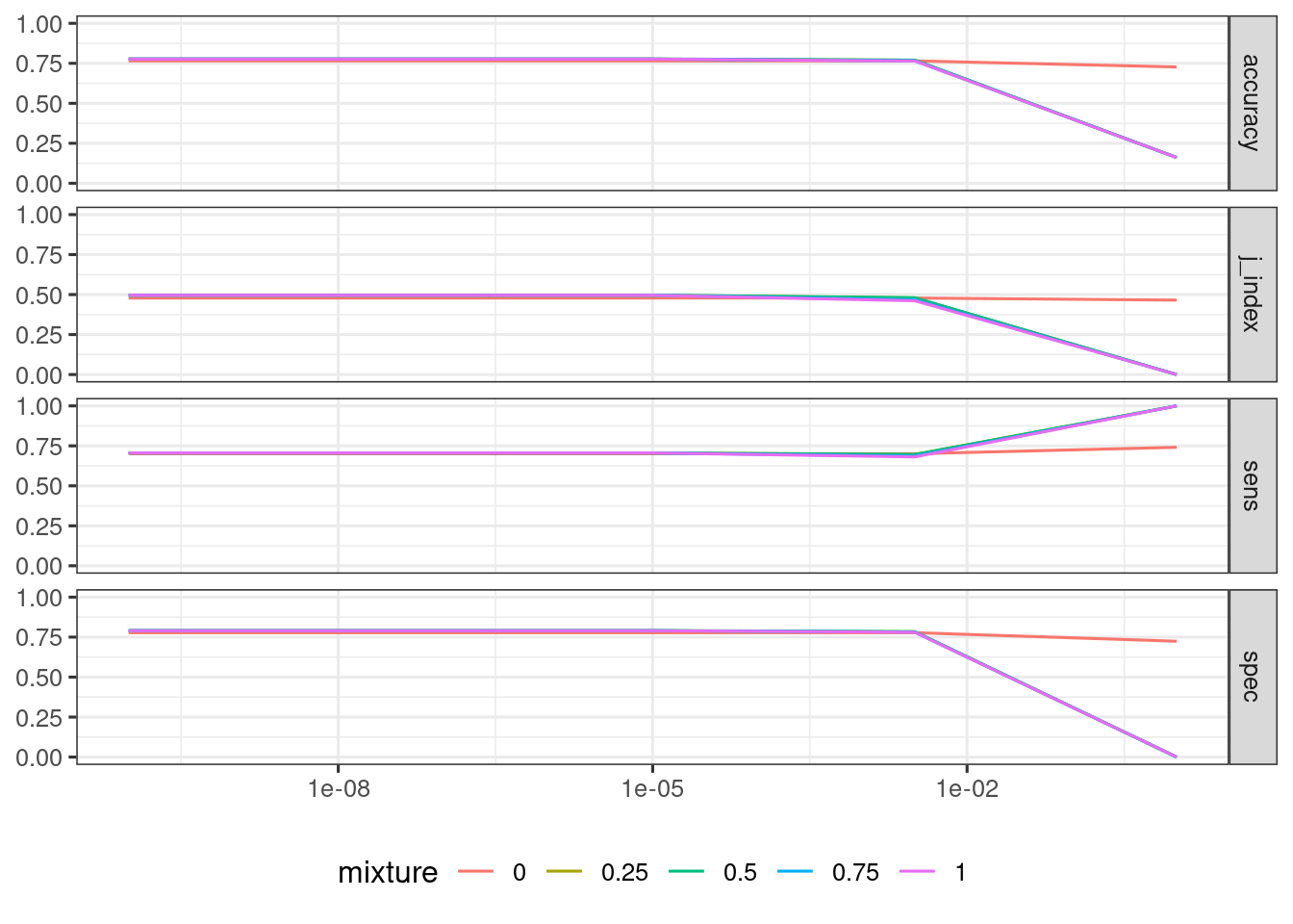
Let’s list the best results of oversampling with tune::show_best(). Here we are obtaining the specific value of the tuning parameters.
show_best(over_lr_results, metric = "j_index")## # A tibble: 5 × 8
## penalty mixture .metric .estimator mean n std_err .config
## <dbl> <dbl> <chr> <chr> <dbl> <int> <dbl> <chr>
## 1 0.0000000001 0.5 j_index binary 0.497 6 0.0648 Preprocessor1_Mod…
## 2 0.0000000316 0.5 j_index binary 0.497 6 0.0648 Preprocessor1_Mod…
## 3 0.00001 0.5 j_index binary 0.497 6 0.0648 Preprocessor1_Mod…
## 4 0.0000000001 0.25 j_index binary 0.496 6 0.0645 Preprocessor1_Mod…
## 5 0.0000000316 0.25 j_index binary 0.496 6 0.0645 Preprocessor1_Mod…With tune::select_best() we pick the best values of hyperparameters.
lr_best <- over_lr_results |>
  select_best(metric = "j_index")
lr_best
## # A tibble: 1 × 3
## penalty mixture .config
## <dbl> <dbl> <chr>
## 1 0.0000000001 0.5 Preprocessor1_Model11The functions tune::show_best() and tune::select_best() work with workflows only, that’s why it is convenient to extract the best workflow from the set.
Let’s fit the final model:
lr_final_model <- fit_best(over_lr_results, metric = "j_index")The metrics on the test set are:
lr_final_model |>
  predict(testing(at_split)) |>
  bind_cols(testing(at_split)) |>
  class_metrics(truth = Attrition, estimate = .pred_class)
## # A tibble: 4 × 3
## .metric .estimator .estimate
## <chr> <chr> <dbl>
## 1 accuracy binary 0.783
## 2 sens binary 0.806
## 3 spec binary 0.778
## 4 j_index binary 0.584As usual, the metrics on the test set are slightly better than with cross validation, as the model is built with the whole train set. Let’s see the confusion matrix:
lr_final_model |>
  predict(testing(at_split)) |>
  bind_cols(testing(at_split)) |>
  conf_mat(truth = Attrition, estimate = .pred_class)
## Truth
## Prediction Yes No
## Yes 29 41
## No 7 144Considering the size of the dataset, the results obtained predicting train and test sets are fairly good. In this kind of problems, it is important to rely on a metric that evaluates sensitivity and specificty simultaneously. If not, it is usual to obain models that assign the same level of the target variable to any testing instance.
References
themiswebsite: https://themis.tidymodels.org/- logistic regression via glmnet https://parsnip.tidymodels.org/reference/details_logistic_reg_glmnet.html.
- technical aspects of the
glmnetmodel https://parsnip.tidymodels.org/reference/glmnet-details.html. - Youden’s J-index https://yardstick.tidymodels.org/reference/j_index.html
Session Info
## R version 4.5.2 (2025-10-31)
## Platform: x86_64-pc-linux-gnu
## Running under: Linux Mint 21.1
##
## Matrix products: default
## BLAS:   /usr/lib/x86_64-linux-gnu/blas/libblas.so.3.10.0
## LAPACK: /usr/lib/x86_64-linux-gnu/lapack/liblapack.so.3.10.0  LAPACK version 3.10.0
##
## locale:
##  [1] LC_CTYPE=es_ES.UTF-8       LC_NUMERIC=C
##  [3] LC_TIME=es_ES.UTF-8        LC_COLLATE=es_ES.UTF-8
##  [5] LC_MONETARY=es_ES.UTF-8    LC_MESSAGES=es_ES.UTF-8
##  [7] LC_PAPER=es_ES.UTF-8       LC_NAME=C
##  [9] LC_ADDRESS=C               LC_TELEPHONE=C
## [11] LC_MEASUREMENT=es_ES.UTF-8 LC_IDENTIFICATION=C
##
## time zone: Europe/Madrid
## tzcode source: system (glibc)
##
## attached base packages:
## [1] stats     graphics  grDevices utils     datasets  methods   base
##
## other attached packages:
##  [1] glmnet_4.1-8       Matrix_1.7-4       themis_1.0.3       yardstick_1.3.2
##  [5] workflowsets_1.1.0 workflows_1.2.0    tune_1.3.0         tidyr_1.3.1
##  [9] tibble_3.3.0       rsample_1.3.0      recipes_1.3.0      purrr_1.2.0
## [13] parsnip_1.3.1      modeldata_1.4.0    infer_1.0.8        ggplot2_4.0.0
## [17] dplyr_1.1.4        dials_1.4.0        scales_1.4.0       broom_1.0.10
## [21] tidymodels_1.3.0
##
## loaded via a namespace (and not attached):
##  [1] tidyselect_1.2.1    timeDate_4041.110   farver_2.1.2
##  [4] S7_0.2.0            fastmap_1.2.0       RANN_2.6.2
##  [7] blogdown_1.21       digest_0.6.37       rpart_4.1.24
## [10] timechange_0.3.0    lifecycle_1.0.4     survival_3.8-6
## [13] magrittr_2.0.4      compiler_4.5.2      rlang_1.1.6
## [16] sass_0.4.10         tools_4.5.2         utf8_1.2.4
## [19] yaml_2.3.10         data.table_1.17.8   knitr_1.50
## [22] prettyunits_1.2.0   labeling_0.4.3      DiceDesign_1.10
## [25] RColorBrewer_1.1-3  withr_3.0.2         nnet_7.3-20
## [28] grid_4.5.2          sparsevctrs_0.3.3   future_1.40.0
## [31] globals_0.17.0      iterators_1.0.14    MASS_7.3-65
## [34] cli_3.6.4           rmarkdown_2.29      generics_0.1.3
## [37] rstudioapi_0.17.1   future.apply_1.11.3 cachem_1.1.0
## [40] splines_4.5.2       parallel_4.5.2      vctrs_0.6.5
## [43] hardhat_1.4.1       jsonlite_2.0.0      bookdown_0.43
## [46] listenv_0.9.1       foreach_1.5.2       gower_1.0.2
## [49] jquerylib_0.1.4     glue_1.8.0          parallelly_1.43.0
## [52] codetools_0.2-19    shape_1.4.6.1       lubridate_1.9.4
## [55] gtable_0.3.6        GPfit_1.0-9         ROSE_0.0-4
## [58] pillar_1.11.1       furrr_0.3.1         htmltools_0.5.8.1
## [61] ipred_0.9-15        lava_1.8.1          R6_2.6.1
## [64] lhs_1.2.0           evaluate_1.0.3      lattice_0.22-5
## [67] backports_1.5.0     bslib_0.9.0         class_7.3-23
## [70] Rcpp_1.1.0          prodlim_2024.06.25  xfun_0.52
## [73] pkgconfig_2.0.3