In this post, I will introduce structural equation modelling (SEM), a statistical technique to evaluate the fit of models including latent and observable variables taking as input the covariance matrix of observable variables.
SEM models can include observable variables (represented with squares in SEM diagrams) and latent variables (represented with circles in SEM diagrams). Latent variables represent constructs not observable directly. Observable variables are supposed to be measurements with error of constructs.
Any SEM model can be split into two submodels:
- Measurement model, specifying the relationship between observable and latent variables.
- Structural model, specifying the relationship between latent variables.
If the model you are examining consists solely of a measurement model, it is a confirmatory factor analysis (CFA) model. CFA is a special case of SEM, where we want to examine the fit of assigning observable variables to specific latent variables.
Let’s see how can we fit SEM models in R. We will use the following packages:
- The
lavaanpackage to fit SEM models. - The
dplyrpackage to handle data frames andpurrto iterate effectively. Those packages belong to the tidyverse. - The
broompackage to present a tidy output oflavaan. semPlotto plot diagrams of SEM models.kableExtrato present nice tables.
library(lavaan)
library(dplyr)
library(purrr)
library(broom)
library(semPlot)
library(kableExtra)
To present the workflow I will use the PoliticalDemocracy dataset included in lavaan. A simpler workflow is presented in the lavaan documentation.
Confirmatory factor analysis
Let’s start examining a m01 model where each observable variable is loading in the latent variable to which is attached theoretically. The latent-observable relationship is specified with a =~, with the latent variable on the left- and the observable variables in the right-hand side.
m01 <- '
  # measurement model
    ind60 =~ x1 + x2 + x3
    dem60 =~ y1 + y2 + y3 + y4
    dem65 =~ y5 + y6 + y7 + y8'
Let’s fit the m01 model usign the lavaan::cfa function, specifying that we are using the PoliticalDemocracy dataset.
f01 <- cfa(m01, data = PoliticalDemocracy)We can use f01 to obtain the path diagram with semPlot::semPaths:
semPaths(f01, edge.label.cex = 0.7, curvePivot = TRUE)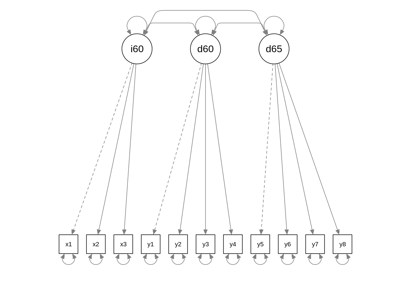
We can learn several things from this plot:
- Note that arrows go from latent to observable variables. This is contrary to general intuition, and means that all latent variables have a common source of variability, the latent variable, and a specific source of variability, introduced in the model as an error term.
- Some of the arrows are presented with a dashed line. This means that the regression coefficient of the observable variable model is set to one. This is done to scale the latent variable.
Let’s examine the output of the lavaan fit of the model. There are three ways of doing this:
summaryfor a summary of selected results.fitMeasuresfor overall fit measures.parameterEstimatesfor a data frame of parameter estimates.
With summary we obtain a report of the model, including selected fit indices and parameter estimates:
summary(f01)## lavaan 0.6-11 ended normally after 47 iterations
##
## Estimator ML
## Optimization method NLMINB
## Number of model parameters 25
##
## Number of observations 75
##
## Model Test User Model:
##
## Test statistic 72.462
## Degrees of freedom 41
## P-value (Chi-square) 0.002
##
## Parameter Estimates:
##
## Standard errors Standard
## Information Expected
## Information saturated (h1) model Structured
##
## Latent Variables:
## Estimate Std.Err z-value P(>|z|)
## ind60 =~
## x1 1.000
## x2 2.182 0.139 15.714 0.000
## x3 1.819 0.152 11.956 0.000
## dem60 =~
## y1 1.000
## y2 1.354 0.175 7.755 0.000
## y3 1.044 0.150 6.961 0.000
## y4 1.300 0.138 9.412 0.000
## dem65 =~
## y5 1.000
## y6 1.258 0.164 7.651 0.000
## y7 1.282 0.158 8.137 0.000
## y8 1.310 0.154 8.529 0.000
##
## Covariances:
## Estimate Std.Err z-value P(>|z|)
## ind60 ~~
## dem60 0.660 0.206 3.202 0.001
## dem65 0.774 0.208 3.715 0.000
## dem60 ~~
## dem65 4.487 0.911 4.924 0.000
##
## Variances:
## Estimate Std.Err z-value P(>|z|)
## .x1 0.082 0.020 4.180 0.000
## .x2 0.118 0.070 1.689 0.091
## .x3 0.467 0.090 5.174 0.000
## .y1 1.942 0.395 4.910 0.000
## .y2 6.490 1.185 5.479 0.000
## .y3 5.340 0.943 5.662 0.000
## .y4 2.887 0.610 4.731 0.000
## .y5 2.390 0.447 5.351 0.000
## .y6 4.343 0.796 5.456 0.000
## .y7 3.510 0.668 5.252 0.000
## .y8 2.940 0.586 5.019 0.000
## ind60 0.448 0.087 5.169 0.000
## dem60 4.845 1.088 4.453 0.000
## dem65 4.345 1.051 4.134 0.000With fitMeasures we obtain a long list of fit indices:
fitMeasures(f01)## npar fmin chisq df
## 25.000 0.483 72.462 41.000
## pvalue baseline.chisq baseline.df baseline.pvalue
## 0.002 730.654 55.000 0.000
## cfi tli nnfi rfi
## 0.953 0.938 0.938 0.867
## nfi pnfi ifi rni
## 0.901 0.672 0.954 0.953
## logl unrestricted.logl aic bic
## -1564.959 -1528.728 3179.918 3237.855
## ntotal bic2 rmsea rmsea.ci.lower
## 75.000 3159.062 0.101 0.061
## rmsea.ci.upper rmsea.pvalue rmr rmr_nomean
## 0.139 0.021 0.428 0.428
## srmr srmr_bentler srmr_bentler_nomean crmr
## 0.055 0.055 0.055 0.060
## crmr_nomean srmr_mplus srmr_mplus_nomean cn_05
## 0.060 0.055 0.055 59.937
## cn_01 gfi agfi pgfi
## 68.225 0.854 0.765 0.531
## mfi ecvi
## 0.811 1.633The output of fitMeasures is a named vector. If we want only some of the fit indices we can do as follows:
fitMeasures(f01, c("npar", "chisq", "tli", "agfi", "rmsea"))## npar chisq tli agfi rmsea
## 25.000 72.462 0.938 0.765 0.101The broom::glance returns a selection of fit indices as a tibble. I use dplyr::select to obtain the selection of fit indices.
glance(f01) |>
  select(npar, chisq, tli, agfi, rmsea)
## # A tibble: 1 × 5
## npar chisq tli agfi rmsea
## <dbl> <dbl> <dbl> <dbl> <dbl>
## 1 25 72.5 0.938 0.765 0.101Finally, with parameterEstimates we obtain a data frame of parameter estimates:
parameterestimates(f01)## lhs op rhs est se z pvalue ci.lower ci.upper
## 1 ind60 =~ x1 1.000 0.000 NA NA 1.000 1.000
## 2 ind60 =~ x2 2.182 0.139 15.714 0.000 1.910 2.454
## 3 ind60 =~ x3 1.819 0.152 11.956 0.000 1.521 2.117
## 4 dem60 =~ y1 1.000 0.000 NA NA 1.000 1.000
## 5 dem60 =~ y2 1.354 0.175 7.755 0.000 1.012 1.696
## 6 dem60 =~ y3 1.044 0.150 6.961 0.000 0.750 1.338
## 7 dem60 =~ y4 1.300 0.138 9.412 0.000 1.029 1.570
## 8 dem65 =~ y5 1.000 0.000 NA NA 1.000 1.000
## 9 dem65 =~ y6 1.258 0.164 7.651 0.000 0.936 1.581
## 10 dem65 =~ y7 1.282 0.158 8.137 0.000 0.974 1.591
## 11 dem65 =~ y8 1.310 0.154 8.529 0.000 1.009 1.611
## 12 x1 ~~ x1 0.082 0.020 4.180 0.000 0.043 0.120
## 13 x2 ~~ x2 0.118 0.070 1.689 0.091 -0.019 0.256
## 14 x3 ~~ x3 0.467 0.090 5.174 0.000 0.290 0.644
## 15 y1 ~~ y1 1.942 0.395 4.910 0.000 1.167 2.717
## 16 y2 ~~ y2 6.490 1.185 5.479 0.000 4.168 8.811
## 17 y3 ~~ y3 5.340 0.943 5.662 0.000 3.491 7.188
## 18 y4 ~~ y4 2.887 0.610 4.731 0.000 1.691 4.083
## 19 y5 ~~ y5 2.390 0.447 5.351 0.000 1.515 3.266
## 20 y6 ~~ y6 4.343 0.796 5.456 0.000 2.783 5.903
## 21 y7 ~~ y7 3.510 0.668 5.252 0.000 2.200 4.819
## 22 y8 ~~ y8 2.940 0.586 5.019 0.000 1.792 4.089
## 23 ind60 ~~ ind60 0.448 0.087 5.169 0.000 0.278 0.618
## 24 dem60 ~~ dem60 4.845 1.088 4.453 0.000 2.713 6.977
## 25 dem65 ~~ dem65 4.345 1.051 4.134 0.000 2.285 6.404
## 26 ind60 ~~ dem60 0.660 0.206 3.202 0.001 0.256 1.065
## 27 ind60 ~~ dem65 0.774 0.208 3.715 0.000 0.366 1.182
## 28 dem60 ~~ dem65 4.487 0.911 4.924 0.000 2.701 6.274Comparing CFA models
Let’s compare the m01 model with two other models:
- A
m00model where all variables are loading in the same factor. - A
m02model where some of the observable variables are allowed to correlate, as specified in the original model. Covariances between variables are specified with a~~operator.
Comparisons between models similar to m00 and m01 are frequently used when reporting CFA analysis. If the confirmatory model works well, it will show a considerably better fit that the one-factor model.
m00 <- '
  #measurement model
    f =~ x1 + x2 + x3 + y1 + y2 + y3 + y4 + y5 + y6 + y7 + y8'

m02 <- '
  # measurement model
    ind60 =~ x1 + x2 + x3
    dem60 =~ y1 + y2 + y3 + y4
    dem65 =~ y5 + y6 + y7 + y8
  # residual correlations
    y1 ~~ y5
    y2 ~~ y4 + y6
    y3 ~~ y7
    y4 ~~ y8
    y6 ~~ y8'
If we need to compare models, it can be a good idea to build an iterative workflow with purrr::map. Let’s start storing the models in a list:
cfa_models <- list(m00, m01, m02)Let’s fit the three models at once:
fit_cfa_models <- map(cfa_models, ~ cfa(., data = PoliticalDemocracy))We can use broom::glance to obtain the selected indices for each model as data frames, and purrr::map_dfr to put them all together in a data frame of three rows:
fit_indices <- map_dfr(fit_cfa_models, ~ glance(.) |> select(npar, chisq, tli, agfi, rmsea))And finally label each model with its name:
fit_indices <- bind_cols(model = c("m00", "m01", "m02"), fit_indices)Here are the results:
fit_indices |>
  kbl() |>
kable_styling(full_width = FALSE)| model | npar | chisq | tli | agfi | rmsea |
|---|---|---|---|---|---|
| m00 | 22 | 255.86259 | 0.6080417 | 0.4486480 | 0.2533787 |
| m01 | 25 | 72.46161 | 0.9375352 | 0.7651101 | 0.1011505 |
| m02 | 31 | 38.12522 | 0.9927314 | 0.8541796 | 0.0345045 |
We observe that the fit of m00 is much poorer than of the other two models. As the degrees of freedom of m02 are smaller than m01, its fit is better. Let’s examine the m02fitted model with semPlot::semPaths.
semPaths(fit_cfa_models[[3]], what = "path", whatLabels = "par", edge.label.cex = 0.7, curvePivot = TRUE)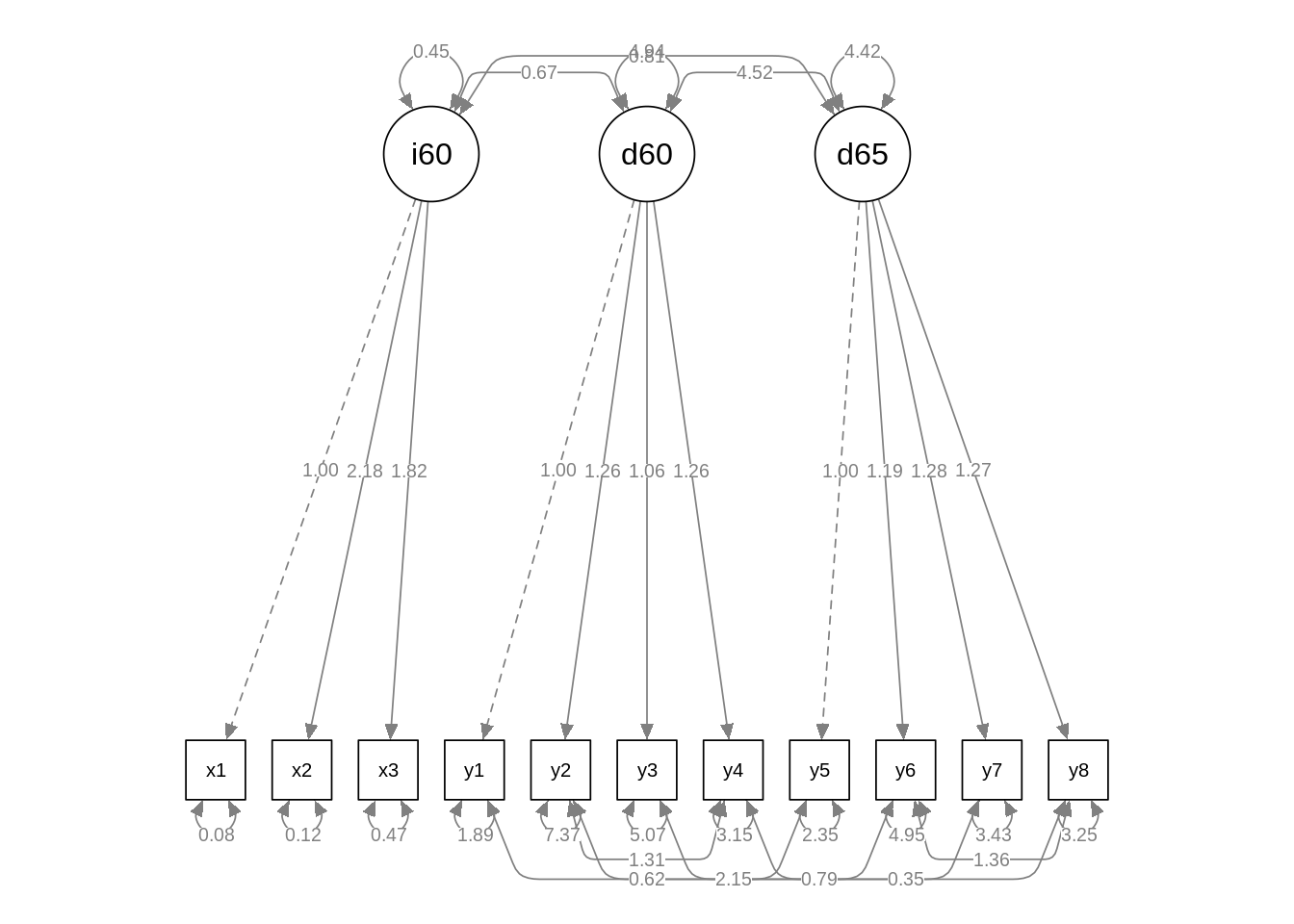
A structural model
Let’s define the structural model presented in the lavaan website. The relationships of the structural model are represented by the ~ symbol.
m03 <- '
  # measurement model
    ind60 =~ x1 + x2 + x3
    dem60 =~ y1 + y2 + y3 + y4
    dem65 =~ y5 + y6 + y7 + y8
  # structural model
    dem60 ~ ind60
    dem65 ~ ind60 + dem60
  # residual correlations
    y1 ~~ y5
    y2 ~~ y4 + y6
    y3 ~~ y7
    y4 ~~ y8
    y6 ~~ y8'
The model can be fit with the lavaan::sem function:
fit_m03 <- sem(m03, data = PoliticalDemocracy)The diagram of this model is:
semPaths(fit_m03, what = "path", whatLabels = "par", edge.label.cex = 0.7, curvePivot = TRUE)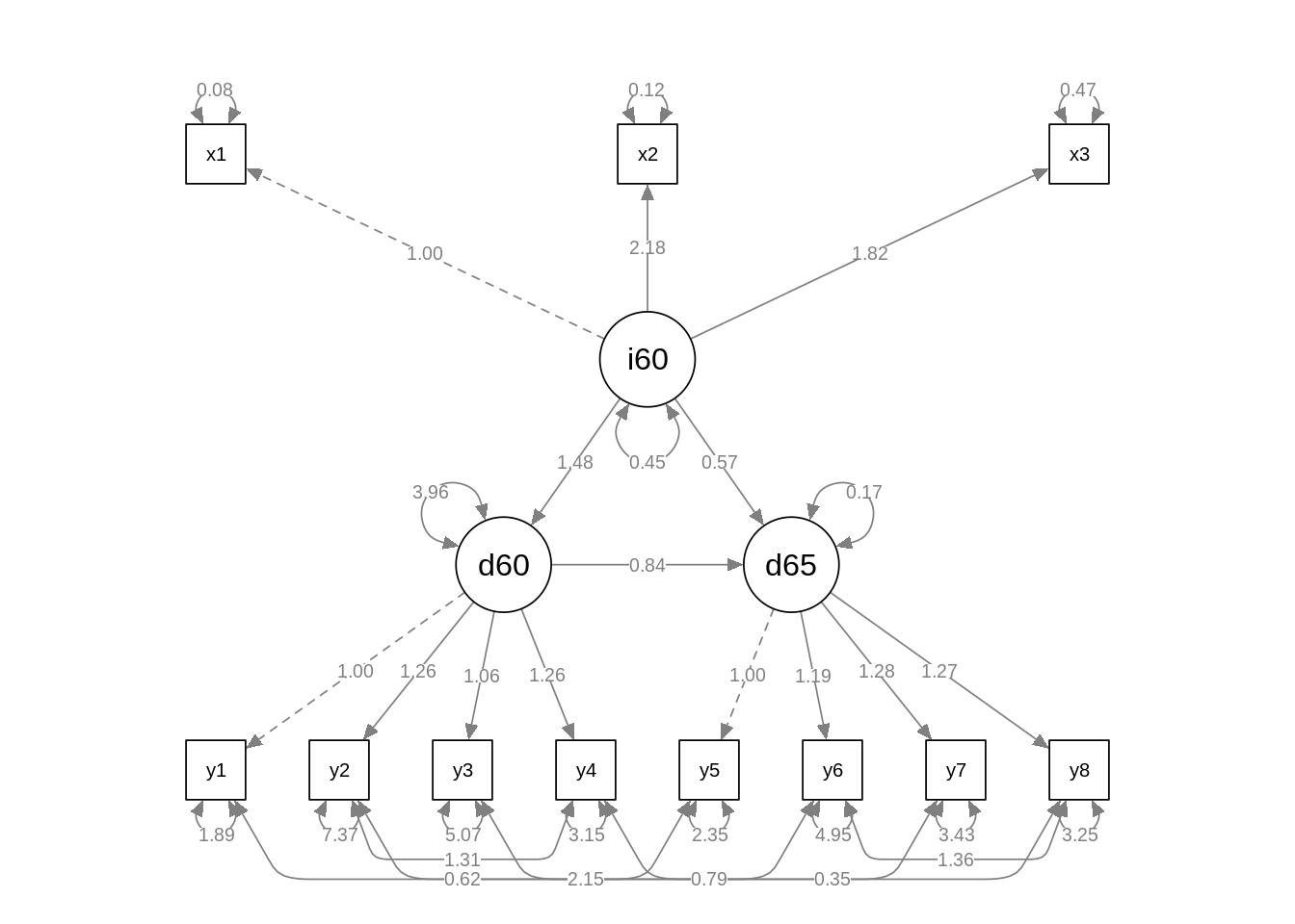
We can use summary, lavaan::fitMeasures and lavaan::parameterEstimates to see the output as with the previous models. Instead of this, I will obtain fit indices in the same way as of previous models, and add the result to the table of CFA fit indices.
df_fit_m03 <- bind_cols(model = "m03", glance(fit_m03) |> select(npar, chisq, tli, agfi, rmsea))

fit_indices <- bind_rows(fit_indices, df_fit_m03)

fit_indices |>
  kbl() |>
kable_styling(full_width = FALSE)| model | npar | chisq | tli | agfi | rmsea |
|---|---|---|---|---|---|
| m00 | 22 | 255.86259 | 0.6080417 | 0.4486480 | 0.2533787 |
| m01 | 25 | 72.46161 | 0.9375352 | 0.7651101 | 0.1011505 |
| m02 | 31 | 38.12522 | 0.9927314 | 0.8541796 | 0.0345045 |
| m03 | 31 | 38.12522 | 0.9927314 | 0.8541796 | 0.0345045 |
We observe that the fit of m02 and m03 is exactly the same.
The parameter estimates are presented as a data table with lavaan, but broom::tidy presents them in a better way as a tibble:
tidy(fit_m03)## # A tibble: 34 × 9
## term op estimate std.error stati…¹ p.value std.lv std.all std.nox
## <chr> <chr> <dbl> <dbl> <dbl> <dbl> <dbl> <dbl> <dbl>
## 1 ind60 =~ x1 =~ 1 0 NA NA 0.670 0.920 0.920
## 2 ind60 =~ x2 =~ 2.18 0.139 15.7 0 1.46 0.973 0.973
## 3 ind60 =~ x3 =~ 1.82 0.152 12.0 0 1.22 0.872 0.872
## 4 dem60 =~ y1 =~ 1 0 NA NA 2.22 0.850 0.850
## 5 dem60 =~ y2 =~ 1.26 0.182 6.89 5.64e-12 2.79 0.717 0.717
## 6 dem60 =~ y3 =~ 1.06 0.151 6.99 2.81e-12 2.35 0.722 0.722
## 7 dem60 =~ y4 =~ 1.26 0.145 8.72 0 2.81 0.846 0.846
## 8 dem65 =~ y5 =~ 1 0 NA NA 2.10 0.808 0.808
## 9 dem65 =~ y6 =~ 1.19 0.169 7.02 2.16e-12 2.49 0.746 0.746
## 10 dem65 =~ y7 =~ 1.28 0.160 8.00 1.33e-15 2.69 0.824 0.824
## # … with 24 more rows, and abbreviated variable name ¹statisticIf we want to check the significance of the coefficients of the structural model, we can do:
tidy(fit_m03) |>
  filter(op == "~") |>
  select(term, estimate, std.error, p.value) |>
  kbl() |>
kable_styling(full_width = FALSE)| term | estimate | std.error | p.value |
|---|---|---|---|
| dem60 ~ ind60 | 1.4830005 | 0.3991486 | 0.0002029 |
| dem65 ~ ind60 | 0.5723362 | 0.2213138 | 0.0097073 |
| dem65 ~ dem60 | 0.8373448 | 0.0983510 | 0.0000000 |
Here we observe that all coefficients are significant for p < 0.001.
The lavaan package is one of the most common packages to fit structural equation models in R. Here I have presented how to retrieve fit indices and parameter estimates from a fitted model, and how to use the broom and purrr functionalities to fit several models at once.
References
- The
lavaantutorial website: https://lavaan.ugent.be/tutorial/ - The
PoliticalDemocracyexample: https://lavaan.ugent.be/tutorial/sem.html - The
semPlotwebsite examples section: http://sachaepskamp.com/semPlot/examples - Mapping with
purrr: https://jmsallan.netlify.app/blog/mapping-with-purrr/
Session info
## R version 4.2.2 Patched (2022-11-10 r83330)
## Platform: x86_64-pc-linux-gnu (64-bit)
## Running under: Linux Mint 19.2
##
## Matrix products: default
## BLAS:   /usr/lib/x86_64-linux-gnu/openblas/libblas.so.3
## LAPACK: /usr/lib/x86_64-linux-gnu/libopenblasp-r0.2.20.so
##
## locale:
##  [1] LC_CTYPE=es_ES.UTF-8       LC_NUMERIC=C
##  [3] LC_TIME=es_ES.UTF-8        LC_COLLATE=es_ES.UTF-8
##  [5] LC_MONETARY=es_ES.UTF-8    LC_MESSAGES=es_ES.UTF-8
##  [7] LC_PAPER=es_ES.UTF-8       LC_NAME=C
##  [9] LC_ADDRESS=C               LC_TELEPHONE=C
## [11] LC_MEASUREMENT=es_ES.UTF-8 LC_IDENTIFICATION=C
##
## attached base packages:
## [1] stats     graphics  grDevices utils     datasets  methods   base
##
## other attached packages:
## [1] kableExtra_1.3.4 semPlot_1.1.5    broom_1.0.1      purrr_0.3.5
## [5] dplyr_1.0.10     lavaan_0.6-11
##
## loaded via a namespace (and not attached):
##   [1] minqa_1.2.4         colorspace_2.0-3    ellipsis_0.3.2
##   [4] htmlTable_2.4.0     corpcor_1.6.10      base64enc_0.1-3
##   [7] rstudioapi_0.13     fansi_1.0.3         xml2_1.3.3
##  [10] splines_4.2.2       mnormt_2.0.2        knitr_1.40
##  [13] glasso_1.11         Formula_1.2-4       jsonlite_1.8.3
##  [16] nloptr_2.0.0        cluster_2.1.4       png_0.1-7
##  [19] compiler_4.2.2      httr_1.4.4          backports_1.4.1
##  [22] assertthat_0.2.1    Matrix_1.5-1        fastmap_1.1.0
##  [25] cli_3.4.1           htmltools_0.5.3     tools_4.2.2
##  [28] igraph_1.3.1        OpenMx_2.20.6       coda_0.19-4
##  [31] gtable_0.3.0        glue_1.6.2          reshape2_1.4.4
##  [34] Rcpp_1.0.9          carData_3.0-5       jquerylib_0.1.4
##  [37] vctrs_0.5.0         svglite_2.1.0       nlme_3.1-161
##  [40] blogdown_1.9        lisrelToR_0.1.4     psych_2.2.3
##  [43] xfun_0.34           stringr_1.4.1       openxlsx_4.2.5
##  [46] lme4_1.1-29         rvest_1.0.3         lifecycle_1.0.3
##  [49] gtools_3.9.2        XML_3.99-0.9        MASS_7.3-58
##  [52] scales_1.2.1        kutils_1.70         parallel_4.2.2
##  [55] RColorBrewer_1.1-3  yaml_2.3.6          pbapply_1.5-0
##  [58] gridExtra_2.3       ggplot2_3.4.0       sass_0.4.1
##  [61] rpart_4.1.19        latticeExtra_0.6-29 stringi_1.7.8
##  [64] highr_0.9           sem_3.1-15          checkmate_2.1.0
##  [67] boot_1.3-28         zip_2.2.0           rlang_1.0.6
##  [70] pkgconfig_2.0.3     systemfonts_1.0.4   arm_1.12-2
##  [73] evaluate_0.17       lattice_0.20-45     htmlwidgets_1.5.4
##  [76] tidyselect_1.1.2    plyr_1.8.7          magrittr_2.0.3
##  [79] bookdown_0.26       R6_2.5.1            generics_0.1.2
##  [82] Hmisc_4.7-0         DBI_1.1.2           pillar_1.8.1
##  [85] foreign_0.8-82      rockchalk_1.8.151   survival_3.4-0
##  [88] abind_1.4-5         nnet_7.3-18         tibble_3.1.8
##  [91] fdrtool_1.2.17      utf8_1.2.2          tmvnsim_1.0-2
##  [94] rmarkdown_2.14      jpeg_0.1-9          grid_4.2.2
##  [97] qgraph_1.9.2        data.table_1.14.2   pbivnorm_0.6.0
## [100] digest_0.6.30       webshot_0.5.3       xtable_1.8-4
## [103] mi_1.0              tidyr_1.2.1         RcppParallel_5.1.5
## [106] stats4_4.2.2        munsell_0.5.0       viridisLite_0.4.1
## [109] bslib_0.3.1