When building a predictive model, it is frequent that observations include spatial attributes such as latitude and longitude. The aim of spatial sampling is to evaluate if a model exhibits poorer performace in some regions of the space. This is implemented in tidymodels with the spatialsample package. Package authors present how the package works in the package website using the ames dataset. In this post, I will show another example of use of this package integrated in the tidymodels workflow using the cat_adoption dataset.
I have also loaded the sf package to create simple features objects from geographical information.
library(tidymodels)
library(spatialsample)
library(sf)
In the cat_adoption dataset, the job consists of predicting if a rescued cat will be returned to its owner or community or transfered to another shelter or dying. Here I am transforming the target variable to factor, and placing the positive case first.
cat_adoption <- cat_adoption |>
  mutate(event = as.factor(event))

levels(cat_adoption$event) <- c("transfered", "returned")

cat_adoption <- cat_adoption |>
  mutate(event = factor(event, levels = c("returned", "transfered")))
We can see that the problem is quite balanced, being the positive case more prevalent than the negative.
cat_adoption |>
  ggplot(aes(event, y = after_stat(count/sum(count)))) +
  geom_bar() +
  labs(title = "Target Variable", x = NULL, y = NULL)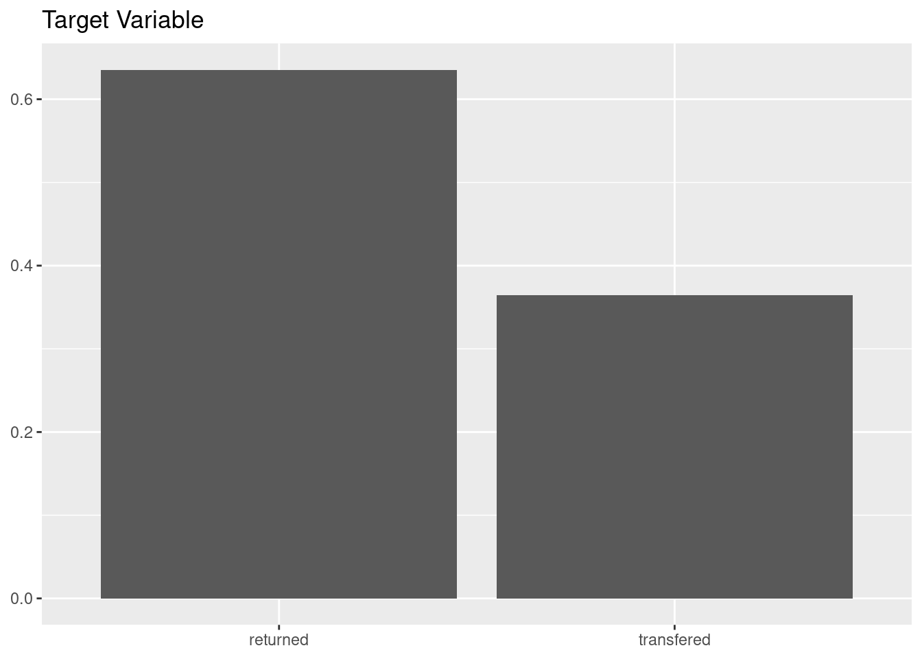
The dataset includes the variables longitude and latitude of the intake or capture of each cat. Here I am plotting the locations of all the cats in the dataset, representing the values of the target variable with different colors. We can see that the target variable is equally distributed across space.
cat_adoption_sf <- st_as_sf(cat_adoption,
                            coords = c("longitude", "latitude"),
                            crs = 4326)

ggplot(cat_adoption_sf) +
  geom_sf(aes(color = event), size = 0.25) +
  labs(title = "Position of cats", x = NULL, y = NULL) +
  scale_color_manual(values = c("red", "blue")) +
  theme_minimal(base_size = 8) +
  theme(legend.position = "bottom")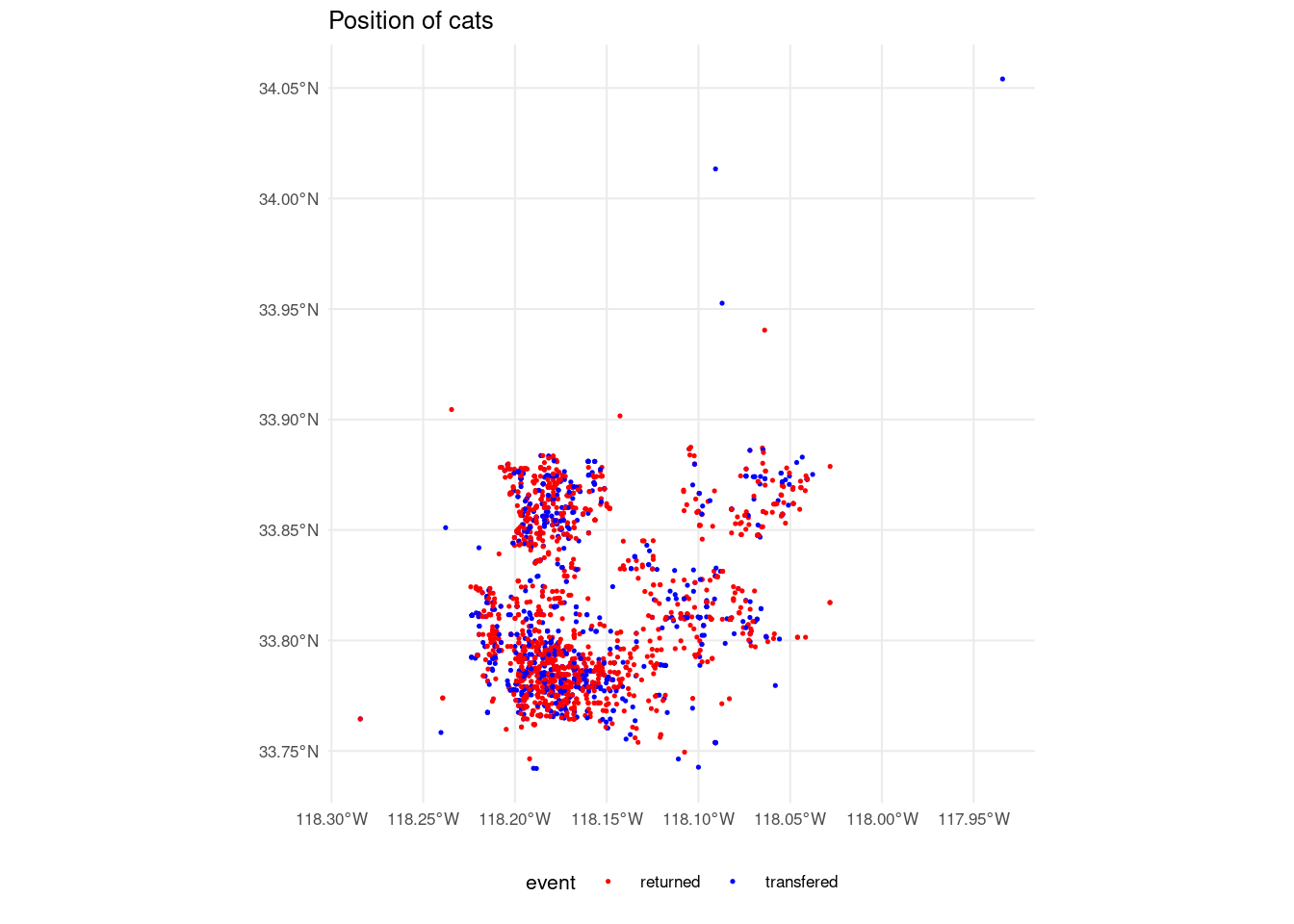
A Decision Tree Model
Let’s define the elements of a tidymodels framework for this job. First, I will split the dataset into train and test with initial_split(). Note that I am using the original cat_adoption dataset without spatial attributes.
set.seed(111)
split <- initial_split(cat_adoption, prop = 0.2, strata = "event")
Secondly, I am defining a recipe. Apart from the step_corr() and step_nzv() correlation and near-zero variance filters, the recipe includes:
- removing
latitudeandlongitude. - collapse low-frequency levels of
intake_conditioninto an other level withstep_other().
rec_cats <- recipe(event ~ ., training(split)) |>
  step_rm(latitude:longitude) |>
  step_corr() |>
  step_nzv() |>
  step_other(intake_condition, threshold = 0.1)
The opportunity of the step_other() recipe comes after exploring the levels of intake_condition.
cat_adoption |>
  ggplot(aes(intake_condition, y = after_stat(count/sum(count)))) +
  geom_bar() +
  labs(title = "Intake Condition", x = NULL, y = NULL)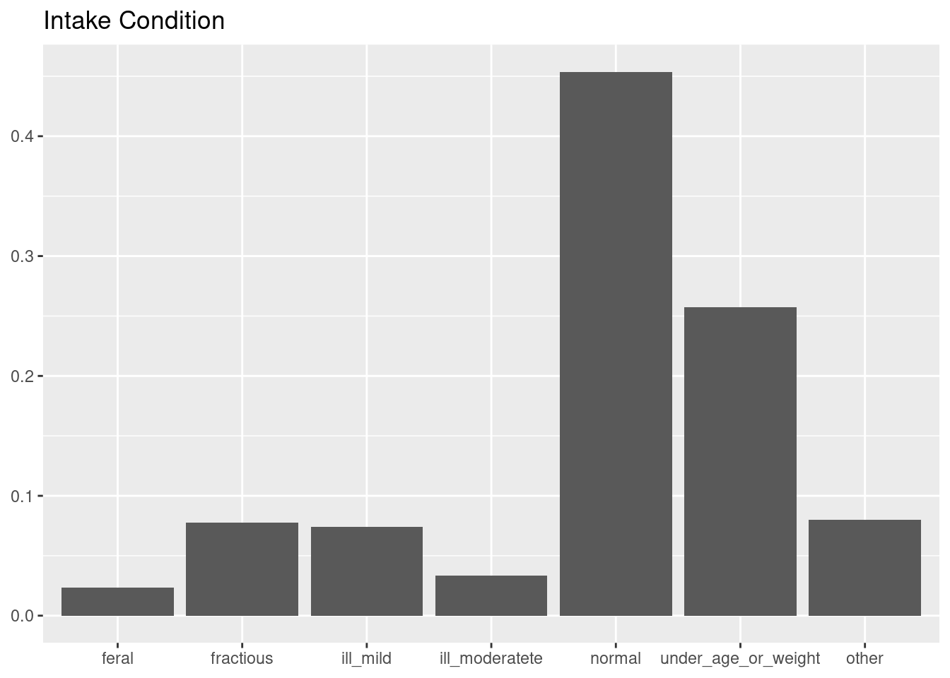
Here is the distribution of intake_condition after applying the recipe.
rec_cats |> prep() |> juice() |>
  ggplot(aes(intake_condition, y = after_stat(count/sum(count)))) +
  geom_bar()  +
  labs(title = "Intake Condition Preprocessed", x = NULL, y = NULL)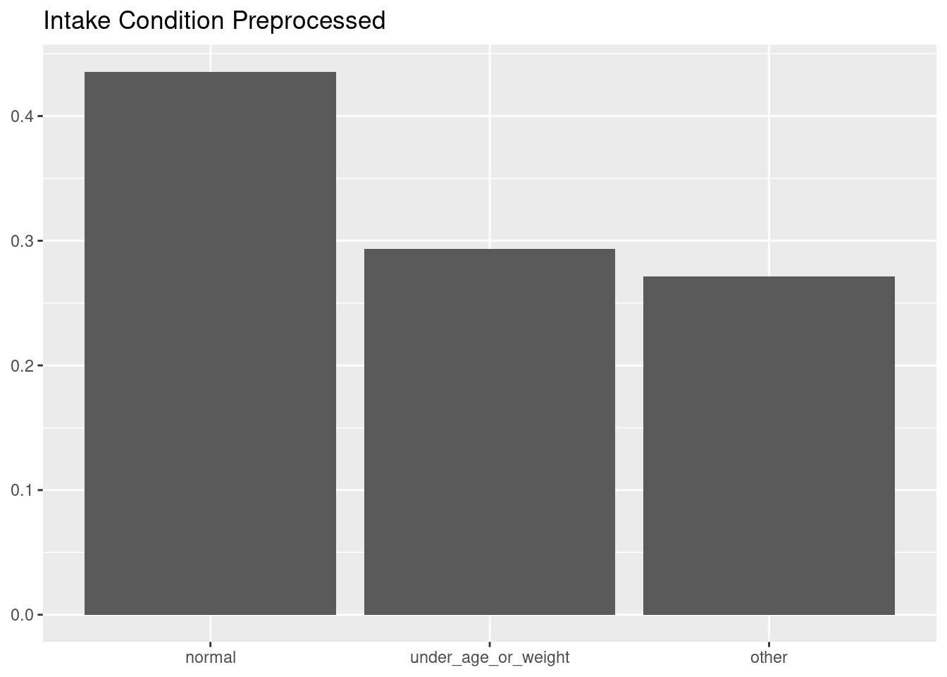
The rest of elements of the modelling framework are:
dt: a decision tree model with the rpart package.folds: a split of the training set into five folds for cross validation.cm: a metric set including accuracy, sensitivity and specificity.
dt <- decision_tree(mode = "classification") |>
  set_engine("rpart")

folds <- vfold_cv(training(split), v = 5, strata = "event")

cm <- metric_set(sens, spec, accuracy)
We can use fit_resamples() to evaluate this model with cross validation.
fit_resamples(object = dt,
              preprocessor = rec_cats,
              resamples = folds,
              metrics = cm) |>
  collect_metrics()
## # A tibble: 3 × 6
## .metric .estimator mean n std_err .config
## <chr> <chr> <dbl> <int> <dbl> <chr>
## 1 accuracy binary 0.820 5 0.0172 Preprocessor1_Model1
## 2 sens binary 0.832 5 0.0307 Preprocessor1_Model1
## 3 spec binary 0.799 5 0.0152 Preprocessor1_Model1In spite of its simplicity, the decision tree model achieves good results in the three classification metrics.
Spatial Resampling
The folds for cross validation defined with vfold_cv() are of similar size and each element is assigned to a fold at random without considering its location. The first step to use spatial resampling is to obtain training_sf, a spatial sf object from the training test. I am using training_sf to apply clustering with spatial_clustering_cv() from spatialsample.
training_sf <- st_as_sf(training(split),
                        coords = c("longitude", "latitude"),
                        crs = 4326, remove = FALSE)

cluster_folds <- spatial_clustering_cv(training_sf, v = 5)
The resamplings of spatialsample have an autoplot() method to represent them.
autoplot(cluster_folds) +
  theme_minimal(base_size = 8) +
  theme(legend.position = "bottom") +
  labs(title = "Spatial Resampling of Traning Set")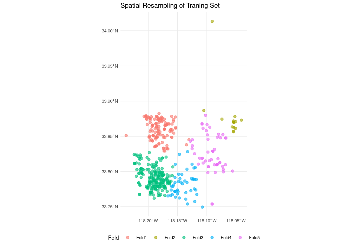
The elements of the training set have been grouped by proximity into clusters. Unlike traditional cross validation, the number of elements of each fold can be different. In this case, peripheral observations are included into less crowded folds.
The aim of spatial resampling is to examine model performance variability across clusters. Then, it does not make sense to average values of metrics across clusters with collect_metrics(). We need to examine the values of metrics in each cluster. We can use fit_resamples() like in cross validation, but using cluster_folds as resamples.
spatial_resamples <- fit_resamples(object = dt,
              preprocessor = rec_cats,
              resamples = cluster_folds,
              metrics = cm)

spatial_resamples
## # Resampling results
## # 5-fold spatial cross-validation
## # A tibble: 5 × 4
## splits id .metrics .notes
## <list> <chr> <list> <list>
## 1 <split [323/127]> Fold1 <tibble [3 × 4]> <tibble [0 × 3]>
## 2 <split [435/15]> Fold2 <tibble [3 × 4]> <tibble [0 × 3]>
## 3 <split [242/208]> Fold3 <tibble [3 × 4]> <tibble [0 × 3]>
## 4 <split [404/46]> Fold4 <tibble [3 × 4]> <tibble [0 × 3]>
## 5 <split [396/54]> Fold5 <tibble [3 × 4]> <tibble [0 × 3]>The result is a tibble with a .metrics column. This column is a list of tibbles, rather than a vector:
spatial_resamples |> pull(.metrics)## [[1]]
## # A tibble: 3 × 4
## .metric .estimator .estimate .config
## <chr> <chr> <dbl> <chr>
## 1 sens binary 0.85 Preprocessor1_Model1
## 2 spec binary 0.745 Preprocessor1_Model1
## 3 accuracy binary 0.811 Preprocessor1_Model1
##
## [[2]]
## # A tibble: 3 × 4
## .metric .estimator .estimate .config
## <chr> <chr> <dbl> <chr>
## 1 sens binary 0.833 Preprocessor1_Model1
## 2 spec binary 0.778 Preprocessor1_Model1
## 3 accuracy binary 0.8 Preprocessor1_Model1
##
## [[3]]
## # A tibble: 3 × 4
## .metric .estimator .estimate .config
## <chr> <chr> <dbl> <chr>
## 1 sens binary 0.856 Preprocessor1_Model1
## 2 spec binary 0.789 Preprocessor1_Model1
## 3 accuracy binary 0.832 Preprocessor1_Model1
##
## [[4]]
## # A tibble: 3 × 4
## .metric .estimator .estimate .config
## <chr> <chr> <dbl> <chr>
## 1 sens binary 0.9 Preprocessor1_Model1
## 2 spec binary 0.812 Preprocessor1_Model1
## 3 accuracy binary 0.870 Preprocessor1_Model1
##
## [[5]]
## # A tibble: 3 × 4
## .metric .estimator .estimate .config
## <chr> <chr> <dbl> <chr>
## 1 sens binary 0.763 Preprocessor1_Model1
## 2 spec binary 0.875 Preprocessor1_Model1
## 3 accuracy binary 0.796 Preprocessor1_Model1Spatial Differences of Metrics
The inspection of the metrics of each cluster reveal some differences of performance. We can consider representing the value of a metric across clusters graphically. Here I have chosen to represent the sensitivity sens. We need to extract the sens row from each cluster and add the results to the training_sf object. For doing that I obtain:
- The assessment sample for each spatial fold, which goes into the
cluster_elementslist. Each element of this list is a spatial object including the observations of the training set belonging to the cluster. - The value of sensitivity for each cluster, which goes into the
cluster_sensvector.
cluster_elements <- map(spatial_resamples |> pull(splits), assessment)
cluster_sens <- map_dbl(spatial_resamples |> pull(.metrics), ~ .|> filter(.metric == "sens") |> pull(.estimate))
I use both objects in map2_dfr() to:
- Attach the value of sensitivity to each element of the cluster.
- Bind the four clusters into a single spatial object.
sens_map <- map2_dfr(cluster_elements, cluster_sens, ~ .x |> mutate(sens = .y))Then, we can plot the training set as a spatial object, coloring each dot according to its value of sensitivity. I have used a gradient scale to represent sensitivity values.
sens_map |>
  ggplot(aes(color = sens)) +
  geom_sf() +
  labs(title = "Sensitivity by Cluster", x = NULL, y = NULL) +
  scale_color_gradient(low = "red", high = "yellow") +
  theme_minimal(base_size = 8) +
  theme(legend.position = "bottom")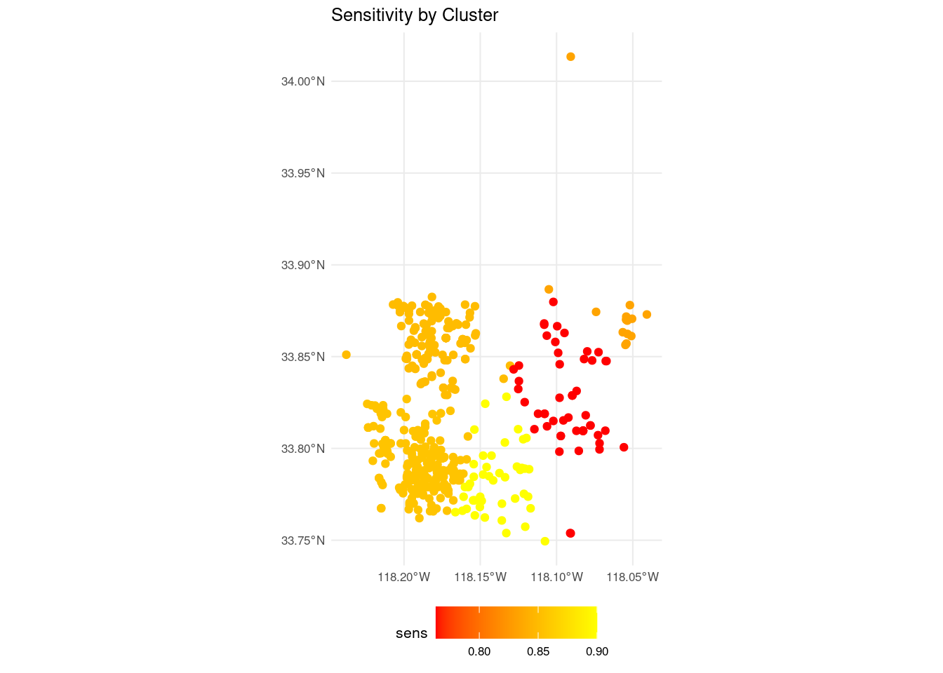
Spatial Resampling
The spatialsample package implements spatial sampling in the tidymodels package. Here I have used clustering to obtain the spatial resample, but there are other methods available, such as spatial blocking, cross validation with buffering or nearest neighbor distance matching. The details for each spatial resampling method can be found in the package website.
This approach benefits from the benefits of the tidyverse, as sf spatial objects can be used in data wrangling functions. This vigneete has shown how to use spatial resampling in a modelling framework including resampling into train and test set and cross validation.
Reference
spatialsamplepackage website: https://spatialsample.tidymodels.org/
Session Info
## R version 4.5.0 (2025-04-11)
## Platform: x86_64-pc-linux-gnu
## Running under: Linux Mint 21.1
##
## Matrix products: default
## BLAS:   /usr/lib/x86_64-linux-gnu/blas/libblas.so.3.10.0
## LAPACK: /usr/lib/x86_64-linux-gnu/lapack/liblapack.so.3.10.0  LAPACK version 3.10.0
##
## locale:
##  [1] LC_CTYPE=es_ES.UTF-8       LC_NUMERIC=C
##  [3] LC_TIME=es_ES.UTF-8        LC_COLLATE=es_ES.UTF-8
##  [5] LC_MONETARY=es_ES.UTF-8    LC_MESSAGES=es_ES.UTF-8
##  [7] LC_PAPER=es_ES.UTF-8       LC_NAME=C
##  [9] LC_ADDRESS=C               LC_TELEPHONE=C
## [11] LC_MEASUREMENT=es_ES.UTF-8 LC_IDENTIFICATION=C
##
## time zone: Europe/Madrid
## tzcode source: system (glibc)
##
## attached base packages:
## [1] stats     graphics  grDevices utils     datasets  methods   base
##
## other attached packages:
##  [1] rpart_4.1.24        sf_1.0-20           spatialsample_0.6.0
##  [4] yardstick_1.3.2     workflowsets_1.1.0  workflows_1.2.0
##  [7] tune_1.3.0          tidyr_1.3.1         tibble_3.2.1
## [10] rsample_1.3.0       recipes_1.3.0       purrr_1.0.4
## [13] parsnip_1.3.1       modeldata_1.4.0     infer_1.0.8
## [16] ggplot2_3.5.2       dplyr_1.1.4         dials_1.4.0
## [19] scales_1.3.0        broom_1.0.8         tidymodels_1.3.0
##
## loaded via a namespace (and not attached):
##  [1] tidyselect_1.2.1    timeDate_4041.110   farver_2.1.2
##  [4] fastmap_1.2.0       blogdown_1.21       digest_0.6.37
##  [7] timechange_0.3.0    lifecycle_1.0.4     survival_3.8-3
## [10] magrittr_2.0.3      compiler_4.5.0      rlang_1.1.6
## [13] sass_0.4.10         tools_4.5.0         utf8_1.2.4
## [16] yaml_2.3.10         data.table_1.17.0   knitr_1.50
## [19] labeling_0.4.3      classInt_0.4-11     DiceDesign_1.10
## [22] KernSmooth_2.23-26  withr_3.0.2         nnet_7.3-20
## [25] grid_4.5.0          sparsevctrs_0.3.3   e1071_1.7-16
## [28] colorspace_2.1-1    future_1.40.0       globals_0.17.0
## [31] iterators_1.0.14    MASS_7.3-65         cli_3.6.4
## [34] rmarkdown_2.29      generics_0.1.3      rstudioapi_0.17.1
## [37] future.apply_1.11.3 proxy_0.4-27        DBI_1.2.3
## [40] cachem_1.1.0        splines_4.5.0       parallel_4.5.0
## [43] s2_1.1.7            vctrs_0.6.5         hardhat_1.4.1
## [46] Matrix_1.7-3        jsonlite_2.0.0      bookdown_0.43
## [49] listenv_0.9.1       foreach_1.5.2       gower_1.0.2
## [52] jquerylib_0.1.4     units_0.8-7         glue_1.8.0
## [55] parallelly_1.43.0   codetools_0.2-19    lubridate_1.9.4
## [58] gtable_0.3.6        munsell_0.5.1       GPfit_1.0-9
## [61] pillar_1.10.2       furrr_0.3.1         htmltools_0.5.8.1
## [64] ipred_0.9-15        lava_1.8.1          R6_2.6.1
## [67] wk_0.9.4            lhs_1.2.0           evaluate_1.0.3
## [70] lattice_0.22-5      backports_1.5.0     bslib_0.9.0
## [73] class_7.3-23        Rcpp_1.0.14         prodlim_2024.06.25
## [76] xfun_0.52           pkgconfig_2.0.3