The maximum network flow problem is a classic problem in graph theory and optimization. It consists of finding the maximum flow that can be sent through a network from a source node to a sink node, subject to capacity constraints on the edges of the network. The network is represented as a directed graph where each edge has a capacity indicating the maximum amount of flow that can pass through it.
The goal of the problem is to determine the maximum amount of flow that can be sent from the source to the sink while satisfying two conditions:
- Conservation of flow: The total amount of flow entering any node must equal the total amount of flow leaving that node.
- Capacity constraints: The amount of flow on any edge cannot exceed its capacity.
The maximum flow problem has numerous real-world applications, including transportation networks, telecommunications, computer networking, and water distribution systems. In this post, I will present how to solve this problem with linear programming using Rglpk, and show how to plot a small instance of the problem with tidygraph and ggraph.
library(Rglpk)
library(tidygraph)
library(ggraph)
Plotting the Instance
Let’s define an instance of the maximum network flow problem. The origin and destination of each arc are stored in org_arcs and dst_arcs, respectively. cap_arcs stores arc capacities, and nodes the graph nodes.
nodes <- c("s", 2:6, "t")
org_arcs <- c(rep("s", 3), 2, 3, rep(4, 3), rep(5, 2), 6)
dst_arcs <- c(2:4, 5, 5, 2, 6, "t", 6, "t", "t")
cap_arcs <- c(3, 5, 3, 3, 3, 2, 2, 4, 5, 3, 2)

network <- data.frame(org = org_arcs,
                      dst = dst_arcs,
                      cap = cap_arcs)
network
## org dst cap
## 1 s 2 3
## 2 s 3 5
## 3 s 4 3
## 4 2 5 3
## 5 3 5 3
## 6 4 2 2
## 7 4 6 2
## 8 4 t 4
## 9 5 6 5
## 10 5 t 3
## 11 6 t 2To plot the graph, we start creating a tidygraph object from the network data frame:
graph <- as_tbl_graph(network)I will present arc capacity between parentheses as edge labels, creating the label1 variable in edges:
graph <- graph |>
  activate(edges) |>
  mutate(label1 = paste0("(", cap, ")"))
graph
## # A tbl_graph: 7 nodes and 11 edges
## #
## # A directed acyclic simple graph with 1 component
## #
## # A tibble: 11 × 4
## from to cap label1
## <int> <int> <dbl> <chr>
## 1 1 2 3 (3)
## 2 1 3 5 (5)
## 3 1 4 3 (3)
## 4 2 5 3 (3)
## 5 3 5 3 (3)
## 6 4 2 2 (2)
## # ℹ 5 more rows
## #
## # A tibble: 7 × 1
## name
## <chr>
## 1 s
## 2 2
## 3 3
## # ℹ 4 more rowsSmall graphs like this require a customised layout, with coordinates of each node stored in a matrix.
ly_mat <- matrix(c(1, 4,
                   3, 3,
                   2, 1,
                   4, 5,
                   5, 2,
                   6, 3,
                   8, 3), 7, 2, byrow = TRUE)
Now we’re ready to plot the graph. Nodes are presented with their name with geom_node_text(), but edges require more work:
- Edge labels are passed as edge aesthetic with
aes(label = label1). - The position of edge labels along the edge and with a specific separation is achieved with
angle_calcandlabel_dodge. - As the graph is directed, we need to specific the aspect of arrows. I do that with the
arrow()instruction. - To avoid overlap between nodes and edges I am setting edge start and end with
start_capandend_cap. - Finally, we specificy
edge_colorout of the aesthetic, because all edges will have the same color.
ggraph(graph, layout = ly_mat) +
  geom_edge_link(aes(label = label1),
                 angle_calc = "along",
                 label_dodge = unit(2.5, "mm"),
                 arrow = arrow(length = unit(4, 'mm'), angle = 20, type = "closed"),
                 start_cap = circle(3, 'mm'),
                 end_cap = circle(3, 'mm'),
                 edge_color = "grey") +
  geom_node_text(aes(label = name)) +
  theme_graph()
## Warning: Using the `size` aesthetic in this geom was deprecated in ggplot2 3.4.0.
## ℹ Please use `linewidth` in the `default_aes` field and elsewhere instead.
## This warning is displayed once every 8 hours.
## Call `lifecycle::last_lifecycle_warnings()` to see where this warning was
## generated.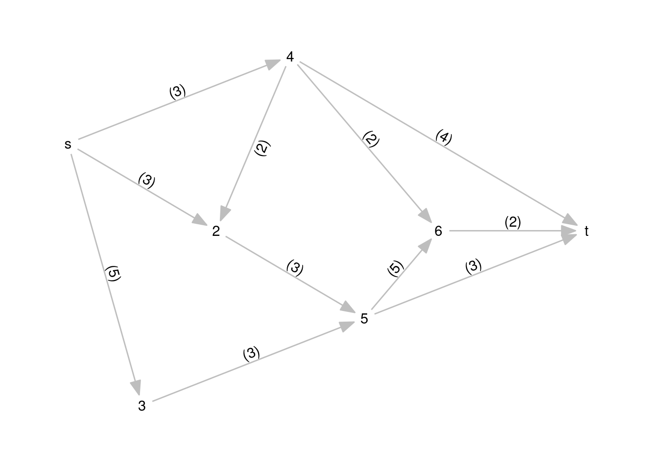
Solving the Instance
The linear programming formulation for the maximum network flow problem requires decision variables \(x_{ij}\), equal to the flow transported through arc from \(i\) to \(j\). The maximum flow to maximize is the variable \(f\). The constraints define flow conservation in each node. Note how variable f appears in the constraint of nodes \(s\) and \(t\). Finally, variables have upper bound arc capacity \(c_{ij}\).
\[\begin{align*} \text{MAX } f \\ \text{s. t. } & x_{s2} + x_{s3} + x_{s4} - f &= 0 \\ & x_{25} - x_{s2} - x_{52} &= 0 \\ & x_{35} - x_{s3} &= 0\\ & x_{42} + x_{46} + x_{4t} - x_{s4} &= 0 \\ & x_{56} + x_{5t} - x_{25} + x_{35} &= 0 \\ & x_{6t} - x_{46} + x_{56} &= 0 \\ & f - x_{47} + x_{5t} + x_{6t} &= 0 \\ & 0 \leq x_{ij} \leq c_{ij} \end{align*}\]
If arc capacities are integer the solution of this problem will be integer, because of the integrality property of network flow problems.
Now we are ready to define all the elements of the linear programming model for the instance:
- Cost coefficients
obj. - Constraints directions
dirand right-hand side valuesrhs. - Variable
types(this could have been omitted in this case as all are continuous) andbounds(note the structure of this variable). - Matrix of constraints coefficients
mat.
n <- length(nodes) #number of rows
m <- length(org_arcs) #number of columns

names_vars <- c(paste0("x[", org_arcs, ", ", dst_arcs, "]"), "flow")
obj <- c(rep(0, m), 1)
names(obj) <- names_vars
dir <- rep("==", n)
rhs <- rep(0, n)
types <- rep("C", m+1)
bounds <- list(upper = list(ind = 1:(m+1), val = c(cap_arcs, Inf)))

rows <- lapply(1:n, \(i){
  orgs <- ifelse(org_arcs == nodes[i], -1, 0)
  dsts <- ifelse(dst_arcs == nodes[i], 1, 0)
  orgs+dsts
})

mat0 <- matrix(unlist(rows), n, m, byrow = TRUE)

mat <- cbind(mat0, c(1, rep(0,n-2), -1))
Once the elements of the problem are defined, we are ready to solve the problem.
sol <- Rglpk_solve_LP(obj = obj,
                      mat = mat,
                      dir = dir,
                      rhs = rhs,
                      bounds = bounds,
                      types = types,
                      max = TRUE)

sol
## $optimum
## [1] 8
##
## $solution
## [1] 3 2 3 3 2 0 0 3 2 3 2 8
##
## $status
## [1] 0
##
## $solution_dual
## [1] 0 0 1 0 0 -1 -1 0 0 1 1 0
##
## $auxiliary
## $auxiliary$primal
## [1] 0 0 0 0 0 0 0
##
## $auxiliary$dual
## [1] 1 1 1 0 1 1 0
##
##
## $sensitivity_report
## [1] NAThe value of maximum flow for this problem is 8. For a better comprehension of the solution, it is useful to present it as a named vector:
solution <- sol$solution
names(solution) <- names_vars
solution
## x[s, 2] x[s, 3] x[s, 4] x[2, 5] x[3, 5] x[4, 2] x[4, 6] x[4, t] x[5, 6] x[5, t]
## 3 2 3 3 2 0 0 3 2 3
## x[6, t] flow
## 2 8Plotting the Solution
Let’s present the solution in the graph plot. To do so, I add the solution to the edges and generate the label2 variable, including the flow and the maximum flow for each edge.
graph <- graph |>
  activate(edges) |>
  mutate(solution = sol$solution[1:m],
         label2 = paste0("(", solution, ", ", cap, ")"))
The graph with the solution shows that the flow is conserved in each node and that maximum capacity is not exceeded in each arc.
ggraph(graph, layout = ly_mat) +
  geom_edge_link(aes(label = label2),
                 angle_calc = "along",
                 label_dodge = unit(2.5, "mm"),
                 arrow = arrow(length = unit(4, 'mm'), angle = 20, type = "closed"),
                 start_cap = circle(3, 'mm'),
                 end_cap = circle(3, 'mm'),
                 edge_color = "grey") +
  geom_node_text(aes(label = name)) +
  theme_graph()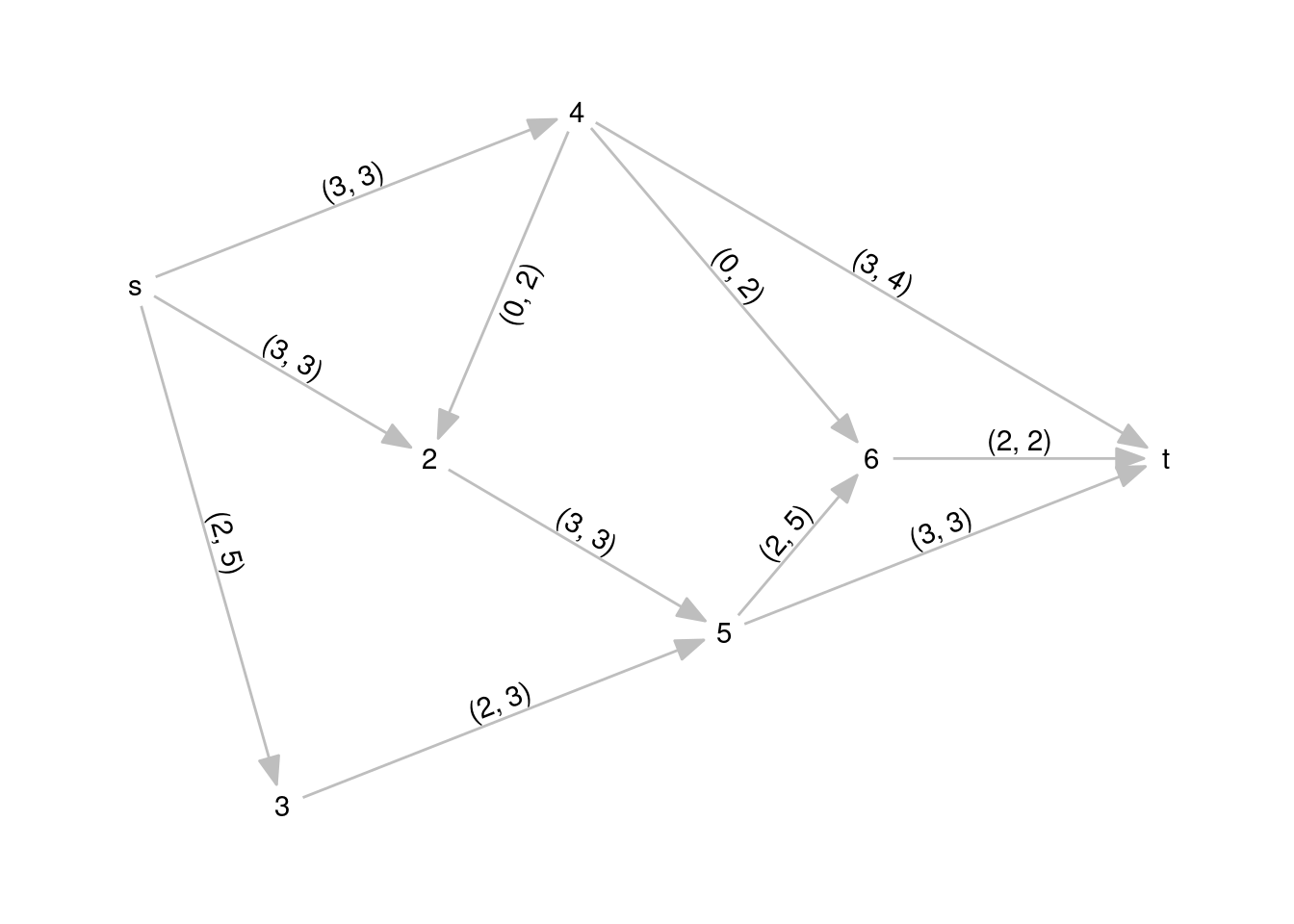
Maximum Flow and Minimum Cut
In graph theory, there is a fundamental relationship between the maximum flow and the minimum cut, known as the max-flow min-cut theorem. This theorem states that in any flow network, the maximum amount of flow passing from the source node to the sink node is equal to the minimum capacity of a cut separating the source node from the sink node.
A cut in a flow network is a partition of the nodes into two sets, one containing the source node and the other containing the sink node, such that there are no edges going from a node in one set to a node in the other set. The capacity of a cut is the sum of the capacities of the edges crossing the cut from the set containing the source node to the set containing the sink node.
The max-flow min-cut theorem implies that the maximum flow in a network is always bounded by the minimum capacity of any cut separating the source from the sink. In other words, the maximum flow value is equal to the capacity of the smallest cut in the network.
For our instance, the minimum cut corresponds with edges (s, 4), (5, t) and (6, 7). This cut creates two subsets of nodes: one with nodes 4 and t and other with the rest of nodes.
To picture this, I define two vectors specifying the cut in edges and nodes.
cut <- rep("no", 11)
names(cut) <- names_vars[1:m]
cut[c(3, 10, 11)] <- "yes"
cut
## x[s, 2] x[s, 3] x[s, 4] x[2, 5] x[3, 5] x[4, 2] x[4, 6] x[4, t] x[5, 6] x[5, t]
## "no" "no" "yes" "no" "no" "no" "no" "no" "no" "yes"
## x[6, t]
## "yes"nodes_cut <- rep("set1", 7)
nodes_cut[c(4,7)] <- "set2"I am adding the cut variables to nodes and edges.
graph <- graph |>
  activate(edges) |>
  mutate(cut = cut)

graph <- graph |>
  activate(nodes) |>
  mutate(cut = nodes_cut)
And finally I am plotting the graph with the minimum cut.
ggraph(graph, layout = ly_mat) +
  geom_edge_link(aes(label = label2, color = cut),
                 angle_calc = "along",
                 label_dodge = unit(2.5, "mm"),
                 arrow = arrow(length = unit(4, 'mm'), angle = 20, type = "closed"),
                 start_cap = circle(3, 'mm'),
                 end_cap = circle(3, 'mm')) +
  geom_node_text(aes(label = name, color = cut)) +
  scale_edge_color_manual(values = c("grey", "#FF0000")) +
  scale_color_manual(values = c("#0000FF", "#FF0000")) +
  theme_graph() +
  theme(legend.position = "none")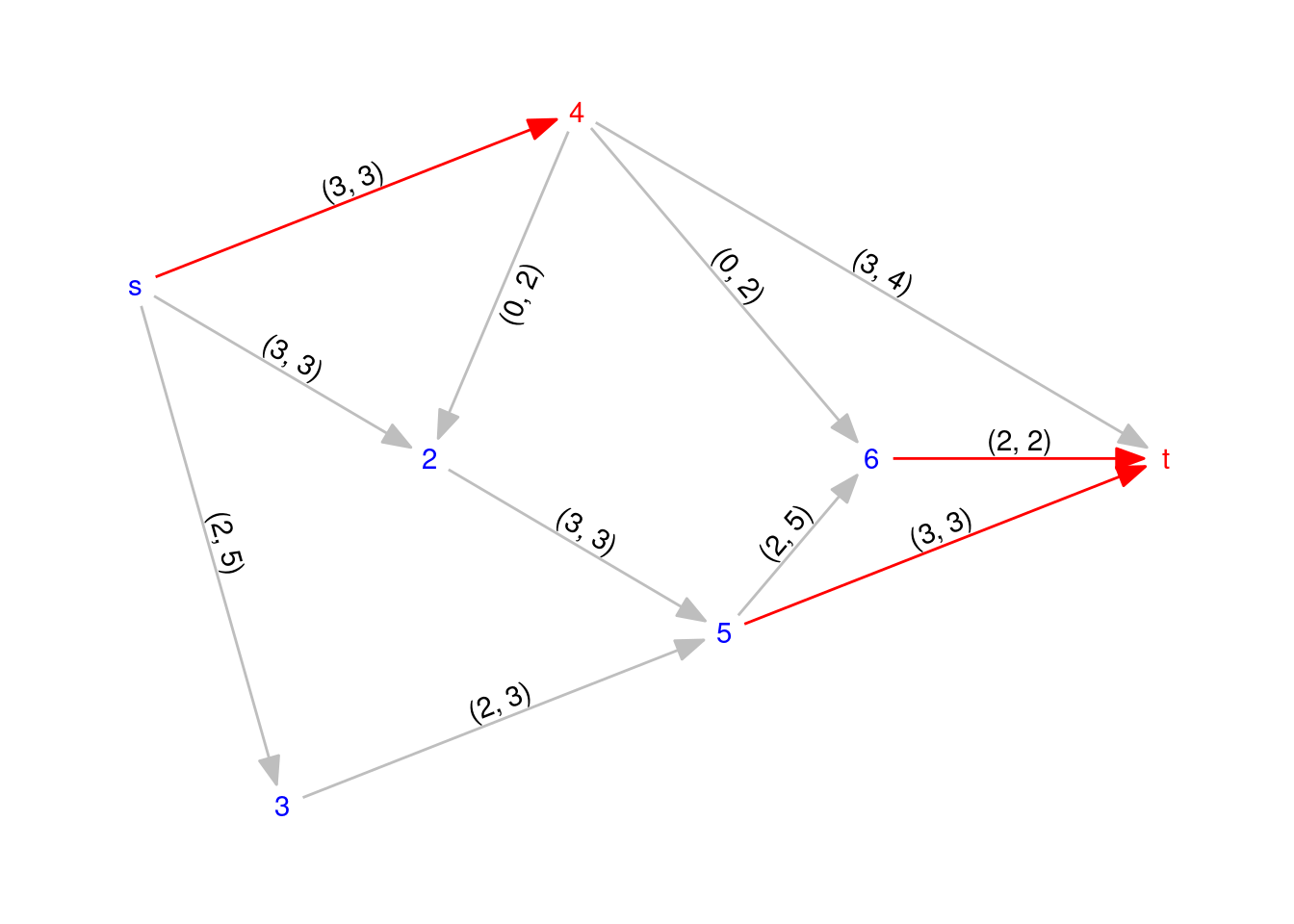
This small example illustrates how to solve the maximum network flow problem with linear programming. This problem can also be solved with specific algorithms, like the Ford-Fulkerson algorithm.
Session Info
## R version 4.3.3 (2024-02-29)
## Platform: x86_64-pc-linux-gnu (64-bit)
## Running under: Linux Mint 21.1
##
## Matrix products: default
## BLAS:   /usr/lib/x86_64-linux-gnu/blas/libblas.so.3.10.0
## LAPACK: /usr/lib/x86_64-linux-gnu/lapack/liblapack.so.3.10.0
##
## locale:
##  [1] LC_CTYPE=es_ES.UTF-8       LC_NUMERIC=C
##  [3] LC_TIME=es_ES.UTF-8        LC_COLLATE=es_ES.UTF-8
##  [5] LC_MONETARY=es_ES.UTF-8    LC_MESSAGES=es_ES.UTF-8
##  [7] LC_PAPER=es_ES.UTF-8       LC_NAME=C
##  [9] LC_ADDRESS=C               LC_TELEPHONE=C
## [11] LC_MEASUREMENT=es_ES.UTF-8 LC_IDENTIFICATION=C
##
## time zone: Europe/Madrid
## tzcode source: system (glibc)
##
## attached base packages:
## [1] stats     graphics  grDevices utils     datasets  methods   base
##
## other attached packages:
## [1] ggraph_2.1.0    ggplot2_3.5.0   tidygraph_1.2.3 Rglpk_0.6-4
## [5] slam_0.1-50
##
## loaded via a namespace (and not attached):
##  [1] viridis_0.6.2      sass_0.4.5         utf8_1.2.3         generics_0.1.3
##  [5] tidyr_1.3.1        blogdown_1.16      digest_0.6.31      magrittr_2.0.3
##  [9] evaluate_0.20      grid_4.3.3         bookdown_0.33      fastmap_1.1.1
## [13] jsonlite_1.8.8     ggrepel_0.9.3      gridExtra_2.3      purrr_1.0.2
## [17] fansi_1.0.4        viridisLite_0.4.1  scales_1.3.0       tweenr_2.0.2
## [21] jquerylib_0.1.4    cli_3.6.1          crayon_1.5.2       graphlayouts_0.8.4
## [25] rlang_1.1.3        polyclip_1.10-4    munsell_0.5.0      withr_2.5.0
## [29] cachem_1.0.7       yaml_2.3.7         tools_4.3.3        dplyr_1.1.4
## [33] colorspace_2.1-0   vctrs_0.6.4        R6_2.5.1           lifecycle_1.0.3
## [37] MASS_7.3-60        pkgconfig_2.0.3    pillar_1.9.0       bslib_0.6.1
## [41] gtable_0.3.3       glue_1.6.2         Rcpp_1.0.10        ggforce_0.4.1
## [45] highr_0.10         xfun_0.39          tibble_3.2.1       tidyselect_1.2.0
## [49] rstudioapi_0.15.0  knitr_1.42         farver_2.1.1       htmltools_0.5.7
## [53] igraph_1.4.2       labeling_0.4.2     rmarkdown_2.21     compiler_4.3.3