When we analyze time series data, we often want to highlight long-term trends and smooth out short-term fluctuations. To accomplish this, we use rolling mean values (sometimes called moving mean). The rolling mean of an observation is the average value of a subset of observations around that observation. If we want of give more importance to specific values of the subset (for instance, those closer in time to the observation), we speak of weighted rolling mean.
In this post, I am introducing how to calculate rolling mean values in R:
- Using the
rollmeanandrollapplyfunctions of thezoopackage together with thedplyrpackage of the tidyverse. - Using the
frollfamily of functions ofdata.table.
I will also load the tidyr and ggplot2 packages for data handling and visualization.
library(ggplot2)
library(dplyr)
library(tidyr)
library(zoo)
library(data.table)
As example of temporal data, I am using the txhousing dataset of ggplot2. This dataset contains information about the housing market in Texas provided by the Texas A&M University real estate center, https://www.recenter.tamu.edu/.
txhousing## # A tibble: 8,602 × 9
## city year month sales volume median listings inventory date
## <chr> <int> <int> <dbl> <dbl> <dbl> <dbl> <dbl> <dbl>
## 1 Abilene 2000 1 72 5380000 71400 701 6.3 2000
## 2 Abilene 2000 2 98 6505000 58700 746 6.6 2000.
## 3 Abilene 2000 3 130 9285000 58100 784 6.8 2000.
## 4 Abilene 2000 4 98 9730000 68600 785 6.9 2000.
## 5 Abilene 2000 5 141 10590000 67300 794 6.8 2000.
## 6 Abilene 2000 6 156 13910000 66900 780 6.6 2000.
## 7 Abilene 2000 7 152 12635000 73500 742 6.2 2000.
## 8 Abilene 2000 8 131 10710000 75000 765 6.4 2001.
## 9 Abilene 2000 9 104 7615000 64500 771 6.5 2001.
## 10 Abilene 2000 10 101 7040000 59300 764 6.6 2001.
## # … with 8,592 more rowsLet’s pick volume of sales in Austin:
volume_Austin <- txhousing %>%
  filter(city == "Austin") %>%
  select(date, volume)
Let’s plot value as a function of date:
ggplot(volume_Austin, aes(date, volume)) +
  geom_line() +
  theme_minimal()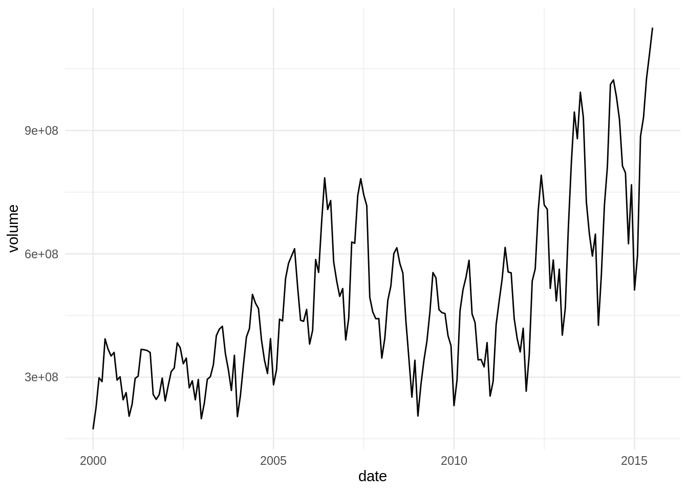
We observe that the volume of sales in the housing market has long-term and short-term fluctuations. Short-term fluctuations have a period of around one year, showing the stationarity of the housing market. To smooth out those fluctuations, we can take the rolling mean, the mean of several contiguous observations. When calculating rolling values it is good practice to define an odd size of the rolling window, so I will use the 13 values around the observation.
Let’s use the rollmean function, with the following parameters:
- the vector to calculate the rolling mean
- the size of rolling window
k - with
fill = NAwe instruct the function to set NA those observations that cannot be calculated - with
align = "center"(the default) we opt for a centered aligment (see below)
rollmean(volume_Austin$volume, k = 13, fill = NA, align = "center")## [1] NA NA NA NA NA NA 289693951
## [8] 294411822 299860431 300168698 306199743 304165323 303898990 304547688
## [15] 296676204 293061810 289699876 293765729 292201590 297943256 304048124
## [22] 305992565 312216667 312497951 309886225 308471071 301858060 304417194
## [29] 304349341 307205899 299605681 299217985 300395331 299420923 300002509
## [36] 301353344 304859848 311864121 312697875 316061659 314249324 322569321
## [43] 315615541 319954324 327068638 334988460 344010755 357210262 363291980
## [50] 367133489 364585768 363346000 362660469 372350396 366825087 375587177
## [57] 389880036 398125039 409048045 421267516 428455182 438634151 442784754
## [64] 446455819 453738928 465733704 464726051 474931163 495568511 504316813
## [71] 522839041 541681345 551739083 562109723 559630725 560658774 565133481
## [78] 571267555 565553066 570412875 586940991 589976746 604344425 612442488
## [85] 609259330 609968934 591876646 582507008 575428165 571272186 558255554
## [92] 558592730 561913102 553652633 551732656 541976214 526118104 511473795
## [99] 489952511 478527170 462605116 454845734 436617740 431629846 427482912
## [106] 419867609 415065492 411508226 405860782 397219703 389820191 391157337
## [113] 395413716 405034487 396541500 403277918 417102133 430347166 442301860
## [120] 451938059 444210913 435846362 426449359 417678423 407695608 406378800
## [127] 396957645 401441389 411783187 413581053 415544904 421110895 418929021
## [134] 426602881 427405499 431397829 432827241 440052889 430958714 438614356
## [141] 457438408 467881400 484864459 504297395 512231219 523973843 521073953
## [148] 531993951 539007652 554487319 553192881 568785651 592458520 614484769
## [155] 643841385 657277929 672807709 689171225 690511154 700719019 701448614
## [162] 713965417 703461349 714903404 734079890 745770587 760538452 766548275
## [169] 774396535 769308151 760255543 765709729 763851562 777195488 766743064
## [176] 779781369 805542711 821998336 838401988 844137832 853932422 NA
## [183] NA NA NA NA NAWe can see that the first six and the six last observations have NA. This is because observation i is obtained averaging values between 6-i and 6+i, so the first valid index is i=7. That is why these values are equal:
mean(volume_Austin$volume[1:13])## [1] 289693951rollmean(volume_Austin$volume, k = 13, fill = NA, align = "center")[7]## [1] 289693951Usually it makes more sense to obtain the i with observations going between i and i-k+1, so we use past values to calculate the rolling value. We achieve this with align = "right".
rollmean(volume_Austin$volume, k = 13, fill = NA, align = "right")## [1] NA NA NA NA NA NA NA
## [8] NA NA NA NA NA 289693951 294411822
## [15] 299860431 300168698 306199743 304165323 303898990 304547688 296676204
## [22] 293061810 289699876 293765729 292201590 297943256 304048124 305992565
## [29] 312216667 312497951 309886225 308471071 301858060 304417194 304349341
## [36] 307205899 299605681 299217985 300395331 299420923 300002509 301353344
## [43] 304859848 311864121 312697875 316061659 314249324 322569321 315615541
## [50] 319954324 327068638 334988460 344010755 357210262 363291980 367133489
## [57] 364585768 363346000 362660469 372350396 366825087 375587177 389880036
## [64] 398125039 409048045 421267516 428455182 438634151 442784754 446455819
## [71] 453738928 465733704 464726051 474931163 495568511 504316813 522839041
## [78] 541681345 551739083 562109723 559630725 560658774 565133481 571267555
## [85] 565553066 570412875 586940991 589976746 604344425 612442488 609259330
## [92] 609968934 591876646 582507008 575428165 571272186 558255554 558592730
## [99] 561913102 553652633 551732656 541976214 526118104 511473795 489952511
## [106] 478527170 462605116 454845734 436617740 431629846 427482912 419867609
## [113] 415065492 411508226 405860782 397219703 389820191 391157337 395413716
## [120] 405034487 396541500 403277918 417102133 430347166 442301860 451938059
## [127] 444210913 435846362 426449359 417678423 407695608 406378800 396957645
## [134] 401441389 411783187 413581053 415544904 421110895 418929021 426602881
## [141] 427405499 431397829 432827241 440052889 430958714 438614356 457438408
## [148] 467881400 484864459 504297395 512231219 523973843 521073953 531993951
## [155] 539007652 554487319 553192881 568785651 592458520 614484769 643841385
## [162] 657277929 672807709 689171225 690511154 700719019 701448614 713965417
## [169] 703461349 714903404 734079890 745770587 760538452 766548275 774396535
## [176] 769308151 760255543 765709729 763851562 777195488 766743064 779781369
## [183] 805542711 821998336 838401988 844137832 853932422We can use the above expression with mutate of dplyr to add a column with the rolling mean.
volume_Austin <- volume_Austin %>%
  mutate(roll_volume = rollmean(volume, k = 13, fill = NA, align = "right"))
Let’s make a temptative plot of the original vaariable and its rolling mean:
volume_Austin %>%
  pivot_longer(-date, names_to = "data", values_to = "volume") %>%
  ggplot(aes(date, volume, color = data)) +
  geom_line() +
  theme_minimal()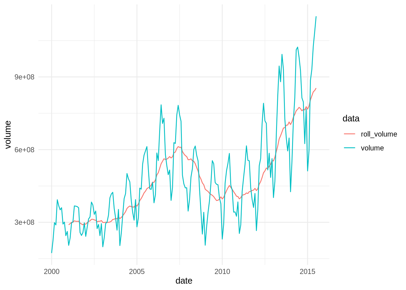
Finally, let’s put it all together from txhousing:
txhousing %>%
  filter(city == "Austin") %>%
  select(date, volume) %>%
  mutate(roll_volume = rollmean(volume, k = 13, fill = NA, align = "right")) %>%
  pivot_longer(-date, names_to = "data", values_to = "volume") %>%
  ggplot(aes(date, volume, color = data)) +
  geom_line() +
  theme_minimal() +
  labs(title = "Volume of housing market (Austin)") +
  scale_color_manual(values = c("#4C9900", "#99FF33"), labels = c("rolled", "straigth")) +
  theme(legend.position = c(0.2, 0.8))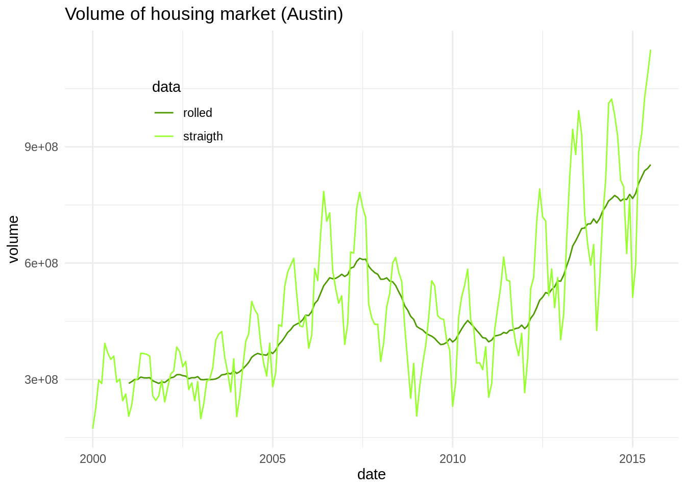
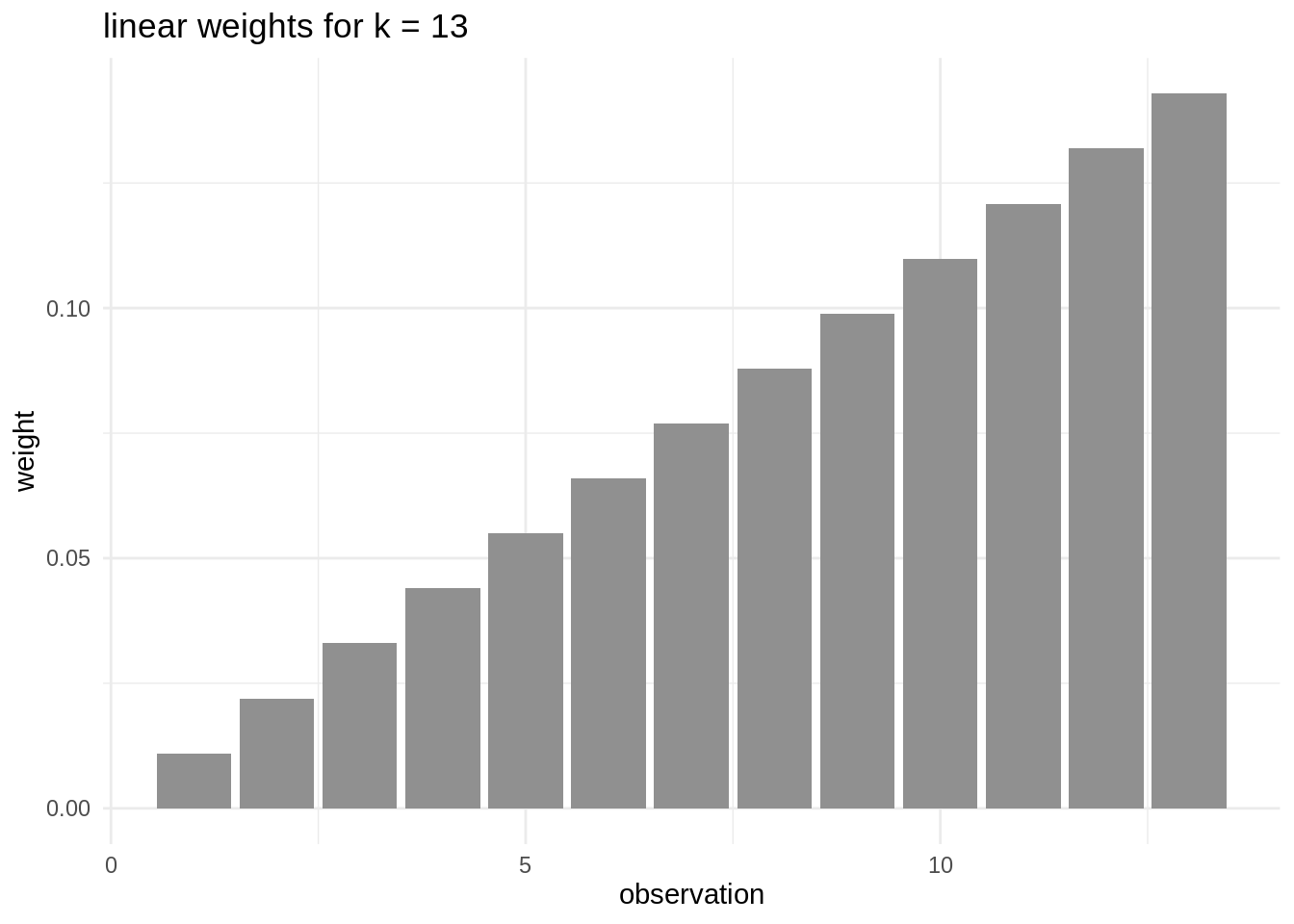
Weighted rolling mean
In some situations, we migth want not to give all observations the same weight when calculating the mean. Instead of giving a weight of 1/k to each observation, we night want to give more weigth to recent observations. We need to define weights so that the summation of them all is equal to one. A possible set of weights is:
weights <- 1:13/sum(1:13)Here is how each of the proposed weights is distributed among observations
To obtain weighted rolling mean, we can use rollapply. This function uses any function to calculate the rolling value. It is more flexible than rollmean, although les computationally efficient.
rollapply(volume_Austin$volume, \(x) sum(weights*x), width = 13, fill = NA, align = "right")## [1] NA NA NA NA NA NA NA
## [8] NA NA NA NA NA 289533067 281631926
## [15] 281983145 282369529 292002795 300635161 309301220 317311706 310651437
## [22] 303385229 298268885 299415945 292031492 290234563 292492562 295078271
## [29] 306147683 314582195 317464468 322685114 317761137 316237779 307739702
## [36] 306315889 290847400 281908661 281295889 281393976 285720803 300154631
## [43] 316653124 333634491 340120982 340840202 333921993 339470749 322529920
## [50] 313917792 315284403 325401207 337313109 359783330 377339240 392123588
## [57] 395477239 392129640 384340286 388760681 375747996 368757367 378121744
## [64] 384811116 405062588 429087853 453869917 480151780 491881223 491245243
## [71] 489727696 491301079 479125370 471868515 487760664 496231697 520971382
## [78] 558399418 582155724 607558752 610143257 606496710 597331754 590252106
## [85] 564423063 547012804 555352904 560881479 582548455 608037742 626753706
## [92] 642173849 625658363 606589695 586528685 567535571 535405218 512061217
## [99] 501811697 496025180 502743563 511754873 516703129 520554573 509975979
## [106] 489387208 456941793 439599342 403980302 381823066 368867004 363204751
## [113] 368792231 388702425 407257687 415603286 424126836 433410600 434840130
## [120] 432135212 407244446 392465073 400744210 414461455 430591597 450869983
## [127] 451162253 449511536 436121902 424180908 410945409 407566829 385799039
## [134] 370389061 374115901 384518894 402386301 430967894 450221509 469480808
## [141] 471836102 467066633 457073335 455092781 430202551 419140964 432738983
## [148] 447860376 481789304 525563106 556200017 584244173 583111559 592250981
## [155] 585565750 588947574 567183052 555087968 568300718 600826889 648032518
## [162] 681777888 729762214 766715609 771971061 766004865 750835670 743188119
## [169] 702068423 680271427 680688314 691998897 730049377 767551295 798342450
## [176] 820145690 826501321 831731074 811571343 812164789 774284611 749839248
## [183] 764981884 783010744 812225475 847695179 891444282Let’s plot the two rolling values in the same plot:
txhousing %>%
  filter(city == "Austin") %>%
  select(date, volume) %>%
  mutate(roll_volume = rollmean(volume, k = 13, fill = NA, align = "right"),
         roll_volume_weighted = rollapply(volume, \(x) sum(weights*x), width = 13, fill = NA, align = "right")) %>%
  pivot_longer(-date, names_to = "data", values_to = "volume") %>%
  ggplot(aes(date, volume, color = data)) +
  geom_line() +
  theme_minimal() +
  labs(title = "Volume of housing market (Austin)") +
  scale_color_manual(values = c("#336600", "#66CC00", "#CCFF99"), labels = c("roll mean", "weighted roll mean", "valume")) +
  theme(legend.position = c(0.2, 0.8))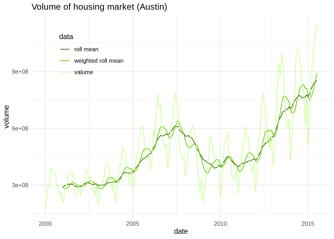
We can see that for this dataset the weighted roll mean has not lost some of the short term fluctuations that are removed in the original roll mean.
Rolling values with data.table
The data.table package includes the froll family of fast rolling functions: frollmean, frollsum and frollapply. Let’s see how can we calculate the same parameters in data.table:
txhousing_dt <- data.table(txhousing)

txhousing_austin <- txhousing_dt[city == "Austin"][ , `:=`(roll_volume = frollmean(volume, n = 13, align = "right"), roll_volume_weighted = frollapply(volume, n = 13, \(x) sum(weights*x), align = "right"))]
Let’s see if zoo and data.table rolling functions return the same values for this dataset:
a <- rollmean(volume_Austin$volume, k = 13, fill = NA, align = "right")
b <- txhousing_austin[, roll_volume]
c <- rollapply(volume_Austin$volume, \(x) sum(weights*x), width = 13, fill = NA, align = "right")
d <- txhousing_austin[, roll_volume_weighted]
identical(a, b)
## [1] TRUEidentical(c, d)## [1] TRUERolled values allow us to tell long-time cycles from short-term fluctuations in time series. The usual choice to obtained rolled values are the rollmean, rollmedian, rollmax, rollsum and rollapply from the zoo package. Users of data.table have available functions frollmean, frollsum and frollaply, optimized for performance and written to be embedded in data table objects.
Session info
## R version 4.1.3 (2022-03-10)
## Platform: x86_64-pc-linux-gnu (64-bit)
## Running under: Linux Mint 19.2
##
## Matrix products: default
## BLAS:   /usr/lib/x86_64-linux-gnu/openblas/libblas.so.3
## LAPACK: /usr/lib/x86_64-linux-gnu/libopenblasp-r0.2.20.so
##
## locale:
##  [1] LC_CTYPE=es_ES.UTF-8       LC_NUMERIC=C
##  [3] LC_TIME=es_ES.UTF-8        LC_COLLATE=es_ES.UTF-8
##  [5] LC_MONETARY=es_ES.UTF-8    LC_MESSAGES=es_ES.UTF-8
##  [7] LC_PAPER=es_ES.UTF-8       LC_NAME=C
##  [9] LC_ADDRESS=C               LC_TELEPHONE=C
## [11] LC_MEASUREMENT=es_ES.UTF-8 LC_IDENTIFICATION=C
##
## attached base packages:
## [1] stats     graphics  grDevices utils     datasets  methods   base
##
## other attached packages:
## [1] data.table_1.14.2 zoo_1.8-9         tidyr_1.1.4       dplyr_1.0.7
## [5] ggplot2_3.3.5
##
## loaded via a namespace (and not attached):
##  [1] highr_0.9        bslib_0.3.0      compiler_4.1.3   pillar_1.6.4
##  [5] jquerylib_0.1.4  tools_4.1.3      digest_0.6.27    lattice_0.20-45
##  [9] jsonlite_1.7.2   evaluate_0.14    lifecycle_1.0.0  tibble_3.1.6
## [13] gtable_0.3.0     pkgconfig_2.0.3  rlang_0.4.12     rstudioapi_0.13
## [17] cli_3.1.0        DBI_1.1.2        yaml_2.2.1       blogdown_1.9
## [21] xfun_0.30        fastmap_1.1.0    withr_2.4.2      stringr_1.4.0
## [25] knitr_1.33       generics_0.1.0   sass_0.4.0       vctrs_0.3.8
## [29] tidyselect_1.1.1 grid_4.1.3       glue_1.4.2       R6_2.5.1
## [33] fansi_0.5.0      rmarkdown_2.13   bookdown_0.26    farver_2.1.0
## [37] purrr_0.3.4      magrittr_2.0.2   scales_1.1.1     htmltools_0.5.2
## [41] ellipsis_0.3.2   assertthat_0.2.1 colorspace_2.0-2 labeling_0.4.2
## [45] utf8_1.2.2       stringi_1.6.2    munsell_0.5.0    crayon_1.4.1