In this plots, I will use information from Instituto Nacional de Estadística (INE), the Spanish official statistical agency, to examine the recent evolution of Spanish inflation. I will use the dplyr functionalities for tabular data handling, and present some functionalities of ggplot2 for presenting plots.
I will be using the tidyverse, lubridate for date handling and kableExtra to present tabular information. I have compiled INE information in the ESdata package.
library(tidyverse)
library(ESdata)
library(lubridate)
library(kableExtra)
INE ellaborates a Consumer Price Index (CPI) on a monthly basis. The inflation between two periods of time is the variation of this index in the reference period. This index has large relevance, as housing rents must be updated yearly according to this index. CPI is calculated using a basket of prices of goods. Those prices are classified in a tree of groups and subgroups. The weight of each group in the CPI is revised yearly.
The ipc_clasif table presents CPI information in tidy format:
ipc_clasif %>%
  slice(1:5) %>%
  kbl() %>%
kable_styling(full_width = FALSE)| periodo | nivel | grupo | dato | valor |
|---|---|---|---|---|
| 2022-09-30 | grupos | general | indice | 109.498 |
| 2022-08-31 | grupos | general | indice | 110.265 |
| 2022-07-31 | grupos | general | indice | 109.986 |
| 2022-06-30 | grupos | general | indice | 110.267 |
| 2022-05-31 | grupos | general | indice | 108.262 |
The variables of this table are:
periodo: The month where data is collected.nivel: The aggregation level of the group for each row. Seeipc_clas_gruposfor the actual meaning of each group.- grupo: The labeo of each group. The label ‘general’ is for the generic inflation data.
dato: The type of datum: ‘index’ is the Consumer Price Index, ‘mensual’ is the monthly inflation rate, ‘anual’ the inter-annual inflation rate and ‘acumulada’ the cumulative inflation rate for the year.valor: The Consumer Price Index For rows with dato equal to ‘indice’, inflation rate in percentage for the rest of values.
Evolution of Spanish inflation
Let’s examine the value of inflation in Spain since 2018. To filter the required data, I am using the year function from lubridate.
Here are some ggplot2 functionalities I have used in this plot:
- The red band covering the COVID lockdown period is made with
geom_rect. I have set some value ofalphaAfter this geom, I have added text withannotate. - The evolution of inflation is presented with
geom_line. I have changed width withsizeand also thecolor. This line is plotted aftergeom_rectto make it visible during the COVID lockdown. - The start of the Ukraine conflict is presented with
geom_vline. I have usedlinetype = "dashed"to present a dashed line. Again, I have usedannotateto add text. If I wanted the line to start at zero, I would have usedgeom_segmentinstead ofgeom_vline. - With
scale_y_continuousI am presenting the inflation as percentage. That’s why I have divided inflationvalueby 100 withmutateat the beginning. I have also set y axis breaks. Withscale_x_date, I am setting a scale break for each year. - With
theme_minimalI set the plot theme, place the legend withlegend.position = "bottom"an annotate the plot withlabs.
ipc_clasif %>%
  filter(year(periodo) >= 2018, grupo == "general", dato == "anual") %>%
  mutate(valor = valor / 100) %>%
  ggplot(aes(periodo, valor)) +
  geom_rect(aes(xmin = as.Date("2020-03-14"), xmax = as.Date("2020-06-21"), ymin = -0.02, ymax = 0.12), fill = "#FF9999", alpha = 0.05) +
  annotate("text", x= as.Date("2019-07-01"), y = 0.06, label = "COVID lockdown", size = 5) +
  geom_line(size = 1, color = "#606060") +
  geom_vline(xintercept = as.Date("2022-02-24"), color = "red", linetype = "dashed", size = 1) +
  annotate("text", x = as.Date("2021-07-01"), y = 0.1, label = "war on Ukraine", size = 5) +
  scale_y_continuous(labels = scales::percent, breaks = seq(-0.02, 0.12, 0.01)) +
  scale_x_date(breaks = scales::date_breaks("1 year"), date_labels = "%Y") +
  theme_minimal() +
  theme(legend.position = "bottom") +
  labs(title = "Evolution of Spanish inflation", x = "time", y = "yearly inflation", caption = "Source: INE")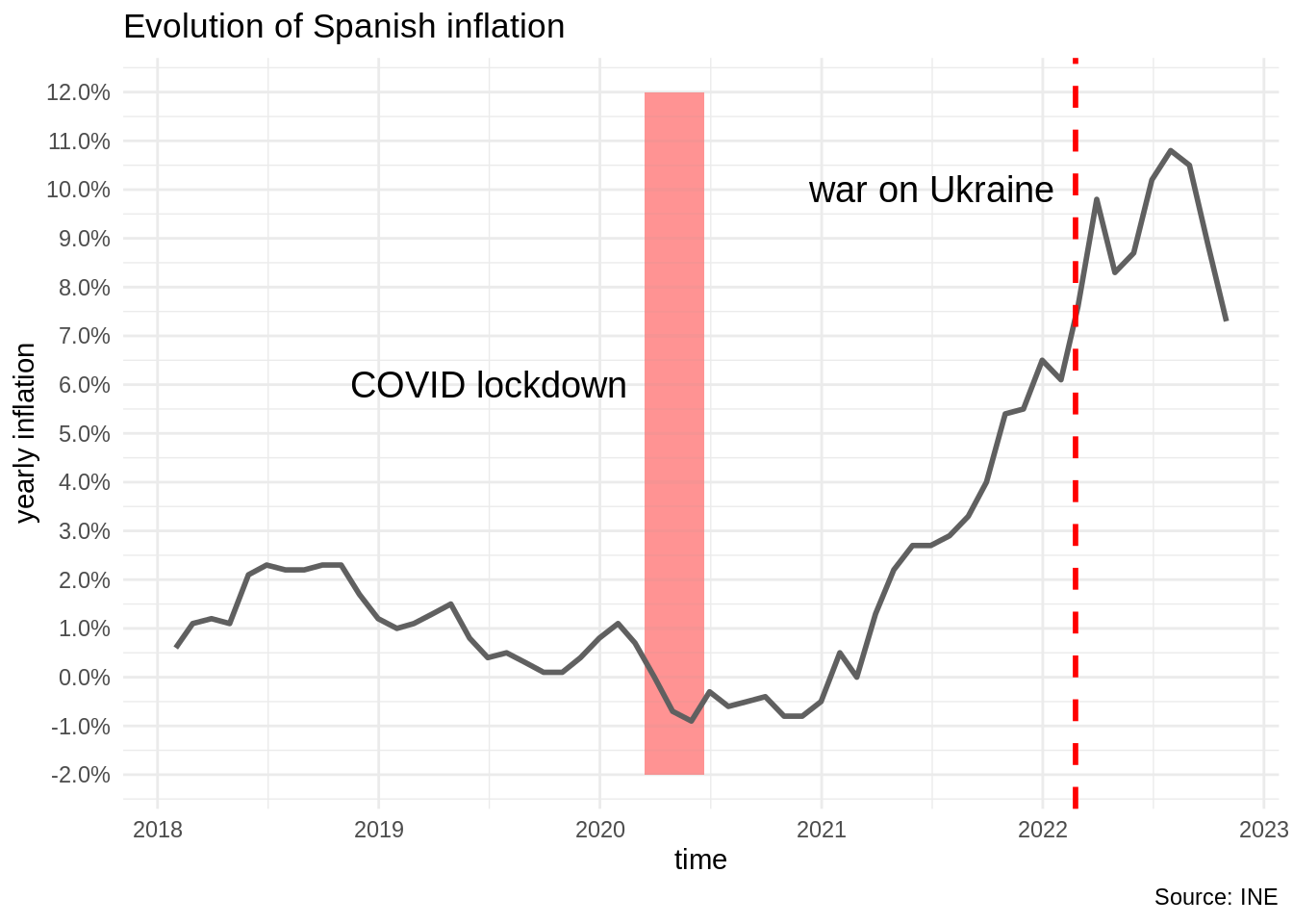
We observe that inflation starts to ramp up at the beginning 2021, some months after the COVID lockdown. The events of Ukraine did not apparently affect inflation. Although yet in high values, it is decreasing since the beginning of 2022.
Evolution of prices of selected groups
Let’s see the groups with largest inflation in the reference period. To do so, I have calculated the maximum value of yearly inflation for each group, and ordered by decreasing value of this maximum:
ipc_ccaa %>%
  filter(region == "ES", year(periodo) >= 2018) %>%
  group_by(grupo) %>%
  summarise(max_value = max(valor)) %>%
  arrange(desc(max_value)) %>%
  slice(1:5) %>%
  kbl() %>%
kable_styling(full_width = FALSE)| grupo | max_value |
|---|---|
| G04 | 125.137 |
| G07 | 119.210 |
| G01 | 114.017 |
| G03 | 111.726 |
| general | 110.267 |
We can see which groups are G04 and G07 with ipc_clas groups:
ipc_clas_grupos %>%
  filter(codigo %in% c("G04", "G07")) %>%
  select(codigo, nombre) %>%
  kbl() %>%
kable_styling(full_width = FALSE)| codigo | nombre |
|---|---|
| G04 | Vivienda, agua, electricidad, gas y otros combustibles |
| G07 | Transporte |
Here is the plot of housing and energy G04, transportation G07 and general index for the same period.
The tricks used here are similar to the plot above, with some differences:
- To make
geom_rectto work correctly, I have set the color parameter. I have chosen the same value asfill. - The ranges of the y axis need to be changed, as prices of groups have more variability than general inflation.
- Color lines and legend values are set with scale_color_manual.
ipc_clasif %>%
  filter(year(periodo) >= 2018, grupo %in% c("general", "G04", "G07"), dato == "anual") %>%
  mutate(valor = valor/100) %>%
  ggplot(aes(periodo, valor, color = grupo)) +
   geom_rect(aes(xmin = as.Date("2020-03-14"), xmax = as.Date("2020-06-21"), ymin = -0.1, ymax = 0.35), fill = "#FF9999", color = "#FF9999", alpha = 0.05) +
  annotate("text", x= as.Date("2019-07-01"), y = 0.15, label = "COVID lockdown", size = 5) +
  geom_line(size = 1) +
  geom_vline(xintercept = as.Date("2022-02-24"), color = "red", linetype = "dashed", size = 1) +
  annotate("text", x = as.Date("2021-07-01"), y = 0.3, label = "war on Ukraine", size = 5) +
  scale_y_continuous(labels = scales::percent) +
  scale_x_date(breaks = scales::date_breaks("1 year"), date_labels = "%Y") +
  scale_color_manual(values = c("#66CC00", "#0080FF", "#606060"), labels = c("energy", "transport", "general"), name = "group") +
  theme_minimal() +
  theme(legend.position = "bottom") +
  labs(title = "Evolution of Spanish inflation (groups)", x = "time", y = "yearly inflation", caption = "Source: INE")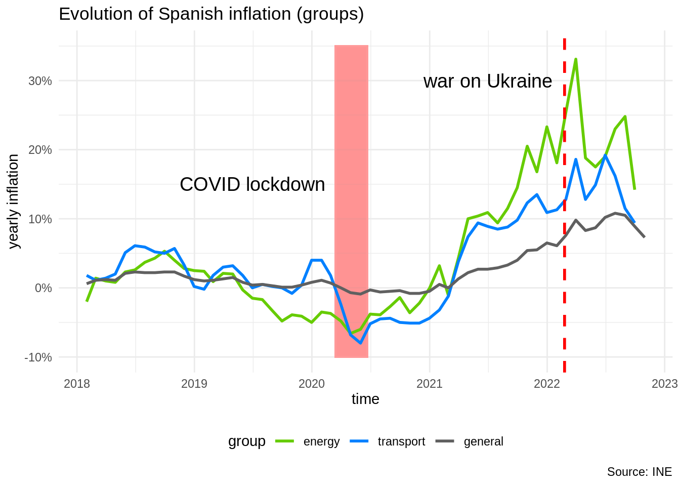
Energy and transportation prices started growing in the middle of the lockdonn, at a higher rate than the global inflation index.
Evolution of prices of electricity and gas
We may be interested in the evolution of gas and electricity. We know that they are in GO45, so we look for these groups with a regular expression using grepl.
ipc_clas_grupos %>%
  filter(grepl("^G045", codigo)) %>%
  select(codigo, nombre) %>%
  kbl() %>%
kable_styling(full_width = FALSE)| codigo | nombre |
|---|---|
| G045 | Electricidad, gas y otros combustibles |
| G0451 | Electricidad |
| G0452 | Gas |
| G0453 | Combustibles líquidos |
| G04510 | Electricidad |
| G04521 | Gas natural y gas ciudad |
| G04522 | Hidrocarburos licuados (butano, propano, etc.) |
| G04530 | Combustibles líquidos |
Here is the evolution of prices of gas G04521 and electricity G04510:
ipc_clasif %>%
  filter(year(periodo) >= 2018, grupo %in% c("general", "G04510", "G04521"), dato == "anual") %>%
  mutate(valor = valor/100) %>%
  ggplot(aes(periodo, valor, color = grupo)) +
  geom_rect(aes(xmin = as.Date("2020-03-14"), xmax = as.Date("2020-06-21"), ymin = -0.2, ymax = 1.2), fill = "#FF9999", color = "#FF9999", alpha = 0.05) +
  annotate("text", x= as.Date("2019-07-01"), y = 0.4, label = "COVID lockdown", size = 5) +
  geom_line(size=1) +
  geom_vline(xintercept = as.Date("2022-02-24"), color = "red", linetype = "dashed", size = 1) +
  annotate("text", x = as.Date("2021-07-01"), y = 0.8, label = "war on Ukraine", size = 5) +
  scale_y_continuous(labels = scales::percent) +
  scale_x_date(breaks = scales::date_breaks("1 year"), date_labels = "%Y") +
  scale_color_manual(values = c("#66CC00", "#0080FF", "#606060"), labels = c("electricity", "gas", "general"), name = "group") +
  theme_minimal() +
  theme(legend.position = "bottom") +
  labs(title = "Evolution of Spanish inflation (gas and electricity)", x = "time", y = "yearly inflation", caption = "Source: INE")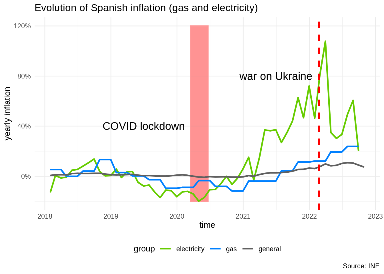
Although the recent events in Ukraine would suggest a rise in the price of gas, it has grown more than electricity prices. Gas and electricity prices started growing earlier than the war in Ukraine. Some people argue, though, that INE considers the evolution of prices or regulated market only. This could reduce the impact of electricity prices in inflation.
References
- The
ESdatapackage. https://github.com/jmsallan/ESdata - Instituto Nacional de Estadística. INEbase. Lista completa de operaciones. https://www.ine.es/dyngs/INEbase/listaoperaciones.htm Accessed 2022-11-12.
- Rodriguez Asensio, D. (2022). Qué está pasando (y qué no) con la inflación en España. https://www.libremercado.com/2022-11-06/daniel-rodriguez-asensio-que-esta-pasando-y-que-no-con-la-inflacion-en-espana-6950646/ Accessed 2022-11-06
Session info
## R version 4.2.2 (2022-10-31)
## Platform: x86_64-pc-linux-gnu (64-bit)
## Running under: Linux Mint 19.2
##
## Matrix products: default
## BLAS:   /usr/lib/x86_64-linux-gnu/openblas/libblas.so.3
## LAPACK: /usr/lib/x86_64-linux-gnu/libopenblasp-r0.2.20.so
##
## locale:
##  [1] LC_CTYPE=es_ES.UTF-8       LC_NUMERIC=C
##  [3] LC_TIME=es_ES.UTF-8        LC_COLLATE=es_ES.UTF-8
##  [5] LC_MONETARY=es_ES.UTF-8    LC_MESSAGES=es_ES.UTF-8
##  [7] LC_PAPER=es_ES.UTF-8       LC_NAME=C
##  [9] LC_ADDRESS=C               LC_TELEPHONE=C
## [11] LC_MEASUREMENT=es_ES.UTF-8 LC_IDENTIFICATION=C
##
## attached base packages:
## [1] stats     graphics  grDevices utils     datasets  methods   base
##
## other attached packages:
##  [1] kableExtra_1.3.4 lubridate_1.8.0  ESdata_0.1.0     forcats_0.5.2
##  [5] stringr_1.4.1    dplyr_1.0.10     purrr_0.3.5      readr_2.1.3
##  [9] tidyr_1.2.1      tibble_3.1.8     ggplot2_3.3.6    tidyverse_1.3.1
##
## loaded via a namespace (and not attached):
##  [1] svglite_2.1.0     assertthat_0.2.1  digest_0.6.30     utf8_1.2.2
##  [5] R6_2.5.1          cellranger_1.1.0  backports_1.4.1   reprex_2.0.2
##  [9] evaluate_0.17     highr_0.9         httr_1.4.4        blogdown_1.9
## [13] pillar_1.8.1      rlang_1.0.6       readxl_1.4.1      rstudioapi_0.13
## [17] jquerylib_0.1.4   rmarkdown_2.14    labeling_0.4.2    webshot_0.5.3
## [21] munsell_0.5.0     broom_1.0.1       compiler_4.2.2    modelr_0.1.9
## [25] xfun_0.34         pkgconfig_2.0.3   systemfonts_1.0.4 htmltools_0.5.3
## [29] tidyselect_1.1.2  bookdown_0.26     fansi_1.0.3       viridisLite_0.4.1
## [33] crayon_1.5.2      tzdb_0.3.0        dbplyr_2.2.1      withr_2.5.0
## [37] grid_4.2.2        jsonlite_1.8.3    gtable_0.3.0      lifecycle_1.0.3
## [41] DBI_1.1.2         magrittr_2.0.3    scales_1.2.1      cli_3.4.1
## [45] stringi_1.7.8     farver_2.1.1      fs_1.5.2          xml2_1.3.3
## [49] bslib_0.3.1       ellipsis_0.3.2    generics_0.1.2    vctrs_0.5.0
## [53] tools_4.2.2       glue_1.6.2        hms_1.1.2         fastmap_1.1.0
## [57] yaml_2.3.6        colorspace_2.0-3  rvest_1.0.3       knitr_1.40
## [61] haven_2.5.1       sass_0.4.1