Random and Scale-Free Network Models

Jose M Sallan 2023-09-13 10 min read

In this post, I will use tidygraph and ggraph to introduce two relevant network models: the Erdős-Renyi model of random networks, and the Barabási-Albert of scale-free networks. I will also use dplyr for tabular data manipulation and igraphdata to get an example of real world network.

library(dplyr)
library(tidygraph)
library(ggraph)
library(igraphdata)

The Erdős-Rényi Model

One of the earliest models of random networks is the Erdős-Rényi (ER) model. There are two equivalent ways of defining the graph of an ER model:

In the \(G\left(n, m \right)\) model, we choose uniformly an element of the set of all graphs of \(n\) nodes and \(m\) edges.
In the \(G\left(n, p\right)\) modeol, each edge of a complete graph of \(n\) nodes can be added with a probability \(p\).

In both formulations nodes are labelled, so that graphs obtained permuting the nodes are considered to be distinct.

We can generate ER graphs with tidygraph using the play_erdos_renyi function. We need to fix n, and we can specify either m or p. We can define an undirected graph of 20 nodes and 100 edges doing:

set.seed(1111)
er <- play_erdos_renyi(n = 20, m = 100, directed = FALSE)

Here is the representation of er using ggraph.

ggraph(er, layout = "kk") +
  geom_node_point(size = 4) +
  geom_edge_link(alpha = 0.5) +
  theme_graph()

## Warning: Using the `size` aesthetic in this geom was deprecated in ggplot2 3.4.0.
## ℹ Please use `linewidth` in the `default_aes` field and elsewhere instead.
## This warning is displayed once every 8 hours.
## Call `lifecycle::last_lifecycle_warnings()` to see where this warning was
## generated.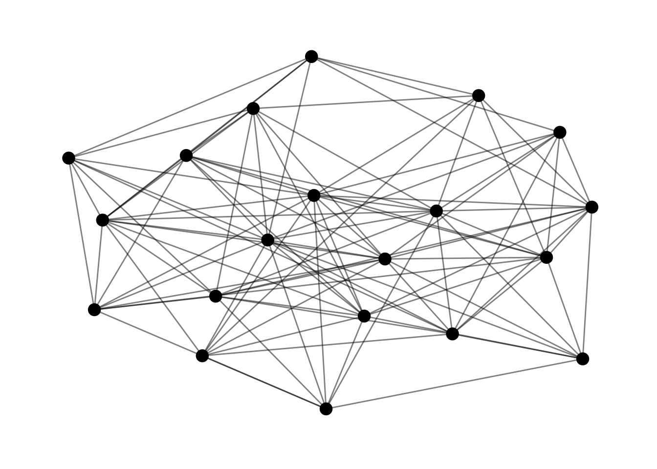

The Degree Distribution of a ER Network

One relevant property of nodes of a graph is the number of nodes to which is connected, known as node degree. The degree of a node \(i\) is usually represented as \(k_i\). Node degree is a relevant measure of centrality or relevance of a node. In a social network, a node with high degree is connected with many nodes of the network and it is supposed to be central or relevant.

The statistical distribution of degree across the nodes of the graph is the **degree *distribution.** This is a relevant property of networks, as it is supposed to be related with network properties, such as connectivity and robustness.

For ER networks, degree distribution follows a binomial distribution of parameters \(n\) and \(p\). For \(n \rightarrow \infty\) and \(np\) finite, node degree tends to a Poisson distribution.

To illustrate this, I have defined a er_deg_distribution function. I am obtaining the degree of each node with contrality_degree(). In the dd table, I am obtaining the probability of each value of degree prob and the probability obtained with a Poisson distribution t_prob. With ggplot I represent the real distribution with a barplot and the theoretical distribution with a line.

er_deg_distribution <- function(graph){
  
  degree <- graph |>
    activate(nodes) |>
    mutate(deg = centrality_degree()) |>
    as_tibble()
  
  av_deg <- mean(degree$deg)
  n_nodes <- nrow(degree)
  n_edges <- graph |> activate(edges) |> as_tibble() |> nrow()
  p <- 2*n_edges/(n_nodes*(n_nodes-1))
  
  dd <- degree |>
    count(deg) |>
    mutate(prob = n/sum(n),
           t_prob = dbinom(deg, n_nodes, p))
  
   dd |>
    ggplot(aes(deg, prob)) +
    geom_bar(stat = "identity", alpha = 0.5) +
    geom_line(aes(deg, t_prob), linewidth = 1.5) +
    theme_minimal() +
    labs(x = "node degree", y = "probability")
  
}

Let’s define a large ER network er2:

set.seed(1111)
er2 <- play_erdos_renyi(n = 1000, p = 0.3, directed = FALSE)

The real and theoretical degree distributions are:

er_deg_distribution(er2)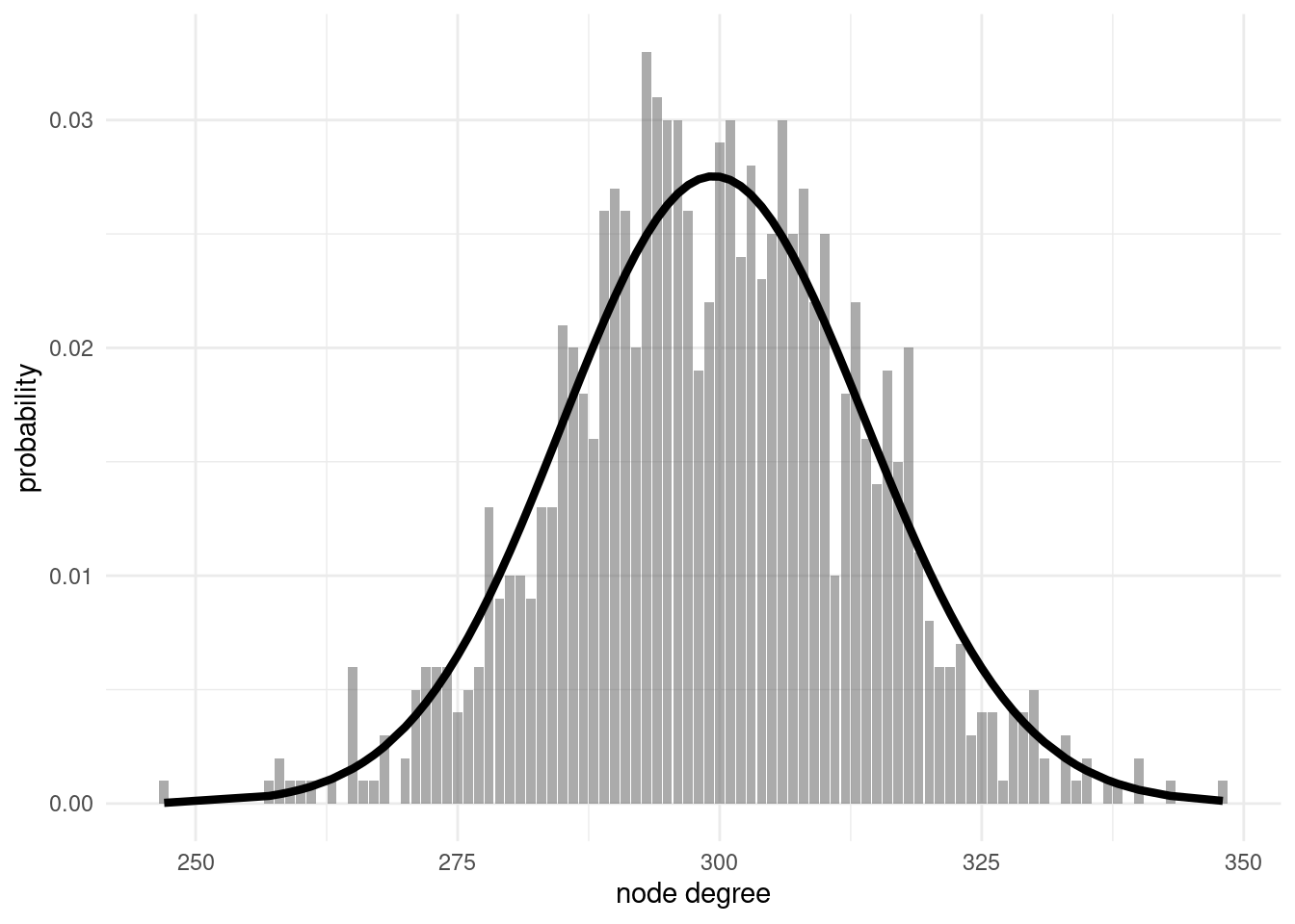

From the figure, we observe that the real and theoretical probability distributions are reasonably similar. From this result, we can describe two relevant properties of degree distribution of ER networks:

Node homogeneity: In the way ER networks are defined, all nodes have similar properties. Each node of a ER network has a degree around to average degree \(\langle k \rangle\).
Exponential decay: As node degree follows a binomial distribution, we cannot expect values of degree much higher than the average. That is what we mean when we say that node degree decays exponentially.

The Barabási-Albert Model of Scale-Free Networks

Many networked system we observe in nature or society have nodes with high degree together with nodes of a small degree. In an airport network, large airports like Frankfurt of Charles de Gaulle have much more connections than regional airports. In a social network, some individuals have much more relationships than the rest of the population. To account for this phenomenon of degree heterogeneity, Barabási and Albert suggested a model of scale-free networks (SF).

SF networks are constructed through two mechanisms: growth and preferential attachment. While the number of nodes and edges of a ER network is fixed beforehand, a SF starts with a complete graph of \(n_0\) nodes, the growth mechanism adds a new node at each stage with \(m \leq n_0\) edges linking it with pre-existing nodes. The preferential attachment mechanism makes the probability of connecting with pre-existing nodes be proportional to node degree. The probability of a new node to connect to a node \(i\) is defined as \(p_i \sim k_i^\alpha + a\). We call \(\alpha\) the power of the preferential attachment and \(a\) the appeal of a node of degree zero.

In tidygraph we can generate a SF network with the play_barabasi_albert function, with the following parameters:

n: number of nodes.
growth: number of edges m to add at each stage.
power: the value of \(\alpha\).
appeal_zero: the value of \(a\).

With the following code we have defined a SF network ba with 20 nodes. Then, I have used centrality_degree() to calculate node degree deg.

set.seed(1111)
ba <- play_barabasi_albert(n = 20, power = 1, 
                           appeal_zero = 0, growth = 5, 
                           directed = FALSE)

ba <- ba |>
  activate(nodes) |>
  mutate(deg = centrality_degree())

Networks built with growth and preferential attachment mechanisms will have node heterogeneity. Nades added in earlier stages will have more probability to be linked with new nodes, and this probability is increased by preferential attachment. In a SF network, a small number of nodes with high degree will coexist with nodes of smaller degree. In this representation of the ba network made with ggraph we observe that all nodes have a degree of at least five, but some nodes have a higher degree.

ggraph(ba, layout = "kk") +
  geom_node_point(aes(size = deg)) +
  geom_edge_link(alpha = 0.5) +
  theme_graph() +
  theme(legend.position = "none")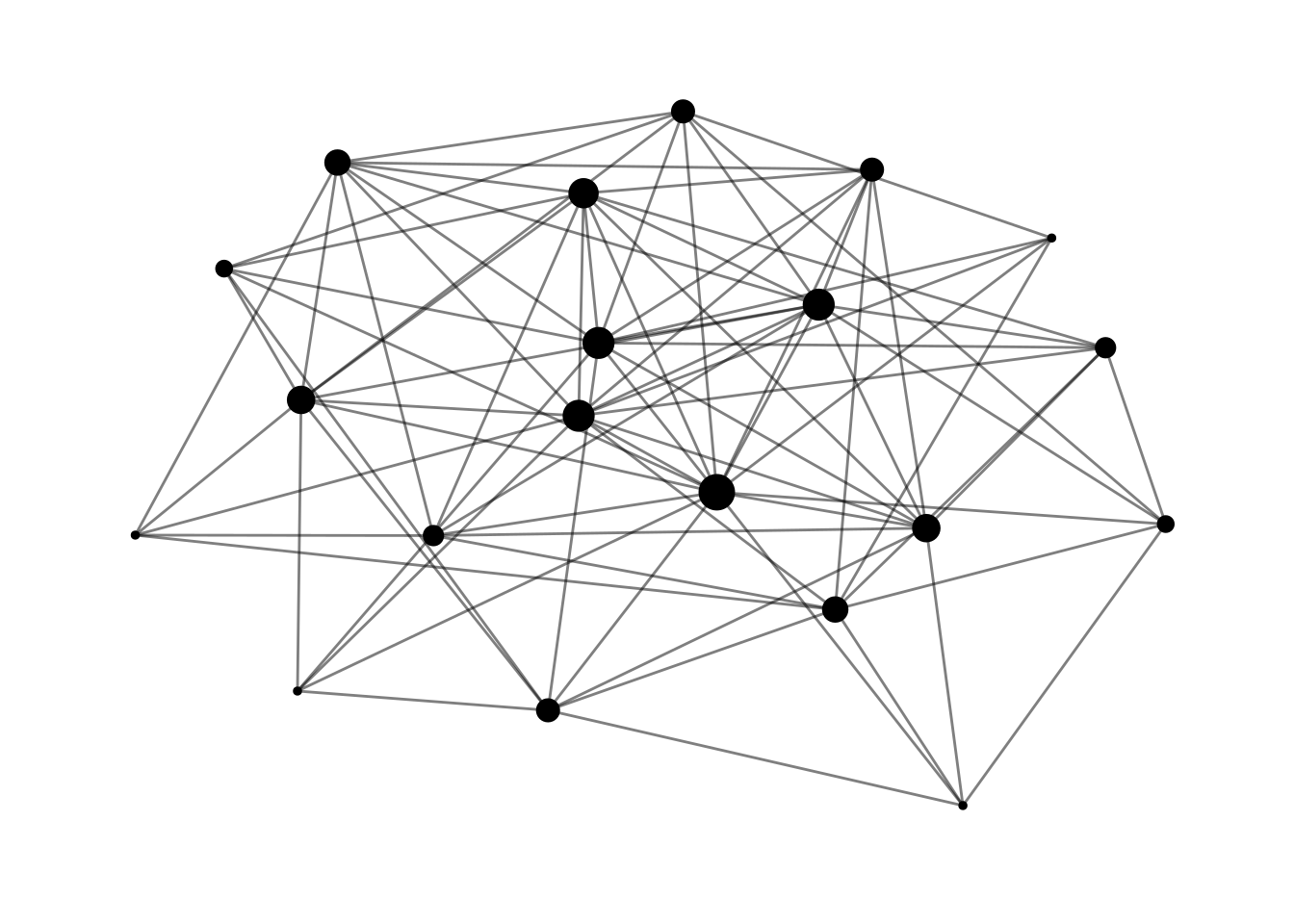

The Degree Distribution of a SF Network

SF networks have a fat-tailed degree distribution, where the probability of finding nodes of high degree is larger than with ER networks. To examine this, I have defined a ba2 network of 1000 nodes:

ba2 <- play_barabasi_albert(n = 1000, power = 1, 
                            appeal_zero = 0, growth = 5, 
                            directed = FALSE)

If we compare the degree distribution of ba2 with the theoretical degree distribution of a ER network, we observe the existence of highly-connected nodes not predicted by the ER model:

er_deg_distribution(ba2)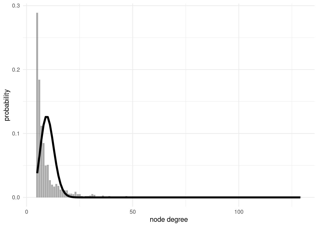

The degree distribution of a SF network is better modeled with a power law, so that the probability of finding nodes of degree k is of the form \(P\left(k\right) \sim k^\gamma\). Power laws are called scale free because they look the same no matter what scale we are examining them. Power laws look as a straight line in a log-log plot, so I have defined a ba_deg_distribution function to represent them.

ba_deg_distribution <- function(graph){
  
  degree <- graph |>
    activate(nodes) |>
    mutate(deg = centrality_degree()) |>
    as_tibble()
  
  dd <- degree |>
    count(deg) |>
    mutate(prob = n / sum(n))
  
  dd |>
    ggplot(aes(deg, prob)) +
    geom_point() +
    theme_minimal() +
    scale_x_log10() +
    scale_y_log10() +
    labs(x = "k", y = "P(k)")
  
}

That’s how the degree distribution of ba2 looks like in the log-log plot:

ba_deg_distribution(ba2)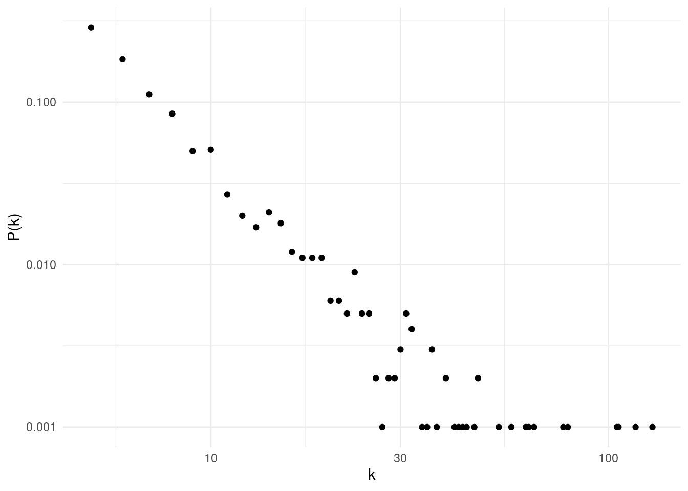

While for low values of degree the distribution looks pretty much like a straight line, for high values of degree the output looks noisy. To remedy this, we usually plot the cumulative degree distribution, defined as \(P_{cum}\left(k\right) = P\left(k' \geq k\right)\). ba_cum_distribution makes the cumulative distribution plot in a log-log scale.

ba_cum_distribution <- function(graph){
  
  degree <- graph |>
    activate(nodes) |>
    mutate(deg = centrality_degree()) |>
    as_tibble()
  
  dd <- degree |>
    count(deg) |>
    arrange(-deg) |>
    mutate(prob = n / sum(n),
           cumprob = cumsum(prob))
  
  dd |>
    ggplot(aes(deg, cumprob)) +
    geom_point() +
    theme_minimal() +
    scale_x_log10() +
    scale_y_log10() +
    labs(x = "k", y = bquote(P[cum](k)))
  
}

That is how the cumulative degree distribution of ba2 looks like:

ba_cum_distribution(ba2)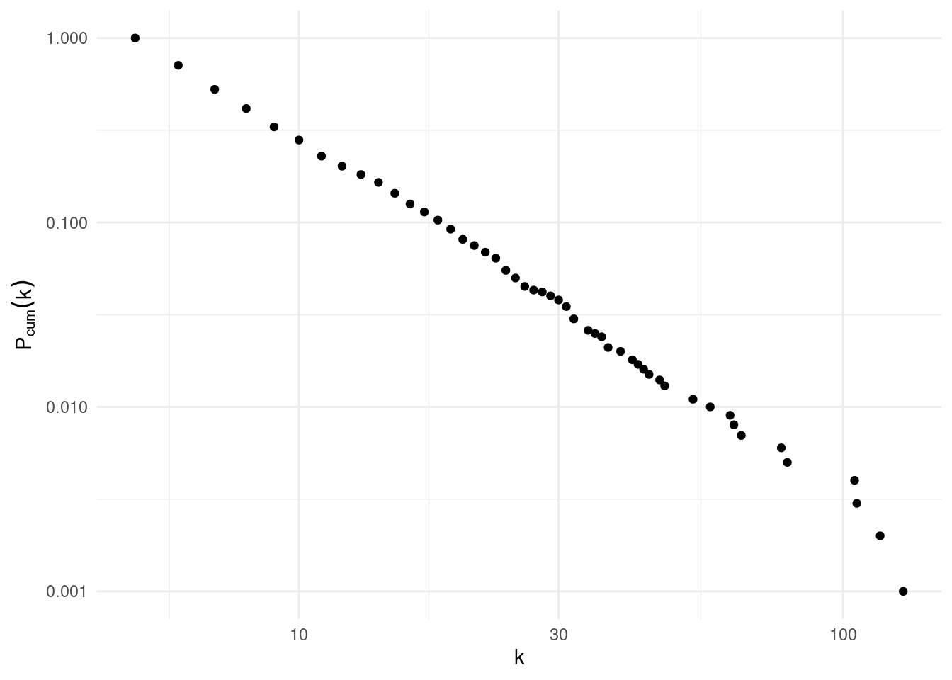

We observe that cumulative degree distribution looks like a straight line with slope \(\gamma_{cum} = \gamma-1\). Those slopes cannot be obtained with least squares regression. If necessary, \(\gamma\) can be calculated using the poweRlaw package.

Degree Distribution of a Real World Network

Let’s see how is the degree distribution of a real world network. I will examine the USairports network from igraphdata.

data("USairports")

In the code below I prepare the data for the analysis using tidygraph:

Defining a tidygraph object us_airports from an igraph object USairports using as_tbl_graph().
The original data included several connections for each pair of airports, so there can be multiple edges between a pair of nodes. We collapse them into a single edge between each pair of nodes with direct connections using to_simple with convert().
The graph has several connected components, and we will analyze the largest connected component us_airports_lcc. We have obtained the nodes belonging to each component with group_components(). We have excluded from the largest connected component the nodes with degree zero.

us_airports <- as_tbl_graph(USairports)

us_airports <- us_airports |>
  convert(to_simple)

us_airports <- us_airports |>
  activate(nodes) |>
  mutate(comp = group_components(),
         d = centrality_degree())

us_airports_lcc <- us_airports |>
  convert(to_subgraph, comp == 1, d > 0)

Here is the cumulative degree distribution of the largest connected component of USairports.

ba_cum_distribution(us_airports_lcc)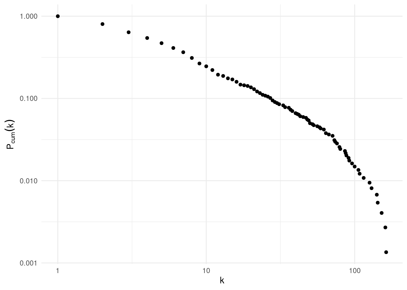

We observe that the degree distribution of the US airport network fits a power law for low values of degree, although we observe a exponential decay for values of degree slightly smaller than 100. This exponential decay appears because the degree predicted for the power law for highly connected nodes is too large for the commercial of technical capabilities of large airports.

Two Network Models

The Erdős-Rényi (ER) model corresponds with the idea that most of us have of a random network, as any pair of nodes can be connected with the same probability. This means that all network nodes have similar statistical properties, one of them being node degree, or the number of nodes to which a node is connected. Many real world networks have node heterogeneity. A network model accounting for node heterogeneity is the scale-free (SF) model. SF networks are created with the mechanisms of growth and preferential attachment, and have a degree distribution that follows a power law. In this scale-free, fat-tailed distribution, there are nodes with a degree much higher than the predicted by the ER model.

References

Adamic, L. Power-laws “scale-free” networks. https://cs.brynmawr.edu/Courses/cs380/spring2013/section02/slides/10_ScaleFreeNetworks.pdf
Barabási, A. L., & Albert, R. (1999). Emergence of scaling in random networks. Science, 286(5439), 509-512.
Erdős, P., & Rényi, A. (1960). On the evolution of random graphs. Publ. Math. Inst. Hung. Acad. Sci, 5(1), 17-60.
poweRlaw: Analysis of Heavy Tailed Distributions. https://cran.r-project.org/web/packages/poweRlaw/index.html

Session Info

sessionInfo()

## R version 4.3.1 (2023-06-16)
## Platform: x86_64-pc-linux-gnu (64-bit)
## Running under: Linux Mint 21.1
## 
## Matrix products: default
## BLAS:   /usr/lib/x86_64-linux-gnu/blas/libblas.so.3.10.0 
## LAPACK: /usr/lib/x86_64-linux-gnu/lapack/liblapack.so.3.10.0
## 
## locale:
##  [1] LC_CTYPE=es_ES.UTF-8       LC_NUMERIC=C              
##  [3] LC_TIME=es_ES.UTF-8        LC_COLLATE=es_ES.UTF-8    
##  [5] LC_MONETARY=es_ES.UTF-8    LC_MESSAGES=es_ES.UTF-8   
##  [7] LC_PAPER=es_ES.UTF-8       LC_NAME=C                 
##  [9] LC_ADDRESS=C               LC_TELEPHONE=C            
## [11] LC_MEASUREMENT=es_ES.UTF-8 LC_IDENTIFICATION=C       
## 
## time zone: Europe/Madrid
## tzcode source: system (glibc)
## 
## attached base packages:
## [1] stats     graphics  grDevices utils     datasets  methods   base     
## 
## other attached packages:
## [1] igraphdata_1.0.1 ggraph_2.1.0     ggplot2_3.4.2    tidygraph_1.2.3 
## [5] dplyr_1.1.2     
## 
## loaded via a namespace (and not attached):
##  [1] viridis_0.6.2      sass_0.4.5         utf8_1.2.3         generics_0.1.3    
##  [5] tidyr_1.3.0        blogdown_1.16      digest_0.6.31      magrittr_2.0.3    
##  [9] evaluate_0.20      grid_4.3.1         bookdown_0.33      fastmap_1.1.1     
## [13] jsonlite_1.8.4     ggrepel_0.9.3      gridExtra_2.3      purrr_1.0.1       
## [17] fansi_1.0.4        viridisLite_0.4.1  scales_1.2.1       tweenr_2.0.2      
## [21] jquerylib_0.1.4    cli_3.6.1          crayon_1.5.2       graphlayouts_0.8.4
## [25] rlang_1.1.0        polyclip_1.10-4    munsell_0.5.0      withr_2.5.0       
## [29] cachem_1.0.7       yaml_2.3.7         tools_4.3.1        colorspace_2.1-0  
## [33] vctrs_0.6.2        R6_2.5.1           lifecycle_1.0.3    MASS_7.3-60       
## [37] pkgconfig_2.0.3    pillar_1.9.0       bslib_0.5.0        gtable_0.3.3      
## [41] glue_1.6.2         Rcpp_1.0.10        ggforce_0.4.1      highr_0.10        
## [45] xfun_0.39          tibble_3.2.1       tidyselect_1.2.0   rstudioapi_0.14   
## [49] knitr_1.42         farver_2.1.1       htmltools_0.5.5    igraph_1.4.2      
## [53] labeling_0.4.2     rmarkdown_2.21     compiler_4.3.1

The Jose M Sallan static website