In this post, I will present a function to implement in base R the Prim’s algorithm to obtain the minimum spanning tree (MST). I will use tidygraph and ggraph to plot the MST of a small graph example.
library(tidygraph)
library(ggraph)
For an undirected and weighted graph \(G\left(N, E \right)\), the MST is a subset of the edges \(E\) that connects all the nodes \(N\) in the graph and with the minimum possible total edge weight. The MST is a problem with practical implications (e.g., wiring a set of cities at minimum cost) and it is also a building block of other algorithms like the Christofides algorithm for the Travelling Salesman Problem.
In the Prim’s algorithm, we cover a node with the MST at each step.
- Step 1. We initialize the set \(L\) of not covered nodes with all the nodes of the graph.
- Step 2. We remove from the set \(L\) an arbitrary node \(n_1\).
- Step 3. We add to the MST the edge \(e\) of minimum weight among those with a node \(i \notin L\) and another node \(j \in L\).
- Step 4. We remove the node \(i\) from the set \(L\).
- Step 5. We return to Step 3 until the set \(L\) is empty.
Prim’s algorithm is a greedy algorithm, which constructs a solution iteratively choosing at each iteration the most appealing element. The MST can be solved optimally with the Prim algorithm.
Building the Function
The prim() function takes as argument a D distance matrix and returns a data frame with rows containing the nodes of each edge. It starts defining the edges table containing the edges ordered by non increasing distance. At each iteration we obtain the positions of the candidate edges cand_edges, and new_edge, the element of cand_edges of minimum distance. The output of the algorithm is the data frame sol_edges.
prim <- function(d){

  n <- dim(d)[1]

  # setting edges
  edges <- data.frame(org = rep(1:n, times = n), dst = rep(1:n, each = n), dist = c(d))
  edges <- edges[which(edges$org != edges$dst), ]
  n_edges <- nrow(edges)
  edges <- edges[order(edges$dist), ]

  # setting vertices
  vertices <- 1:n
  notL <- 1
  sol_edges <- data.frame()

  for(i in 1:(n-1)){

    # candidate edges
    cand_edges <- which(edges$org%in% notL & !edges$dst %in% notL)

    # new edge: first compatible
    new_edge <- edges[cand_edges[1], ]

    #constructing the solution
    sol_edges <- rbind(sol_edges, new_edge)

    #updating set L
    notL <- c(notL, new_edge$dst)

  }

  sol_edges <- sol_edges[, 1:2]
  return(sol_edges)

}
Applying the Function
Let’s define a graph of six nodes with coordinates:
l <- matrix(c(1, 2,
              2, 1,
              3, 2,
              4, 4,
              2, 5,
              4, 6), ncol = 2, byrow = TRUE)
The distance between nodes is obtained as:
d_l <- as.matrix(dist(l))Then, we apply the algorithm to obtain the MST with the prim() function:
p_l <- prim(d_l)
p_l
## org dst
## 7 1 2
## 14 2 3
## 21 3 4
## 34 4 6
## 28 4 5Plotting the MST
We can use the output of the algorithm to define a graph. We will label the nodes with letters A of F.
g_l <- tbl_graph(edges = p_l)
g_l <- g_l |>
  activate(nodes) |>
  mutate(name = LETTERS[1:nrow(l)])
g_l
## # A tbl_graph: 6 nodes and 5 edges
## #
## # A rooted tree
## #
## # Node Data: 6 × 1 (active)
## name
## <chr>
## 1 A
## 2 B
## 3 C
## 4 D
## 5 E
## 6 F
## #
## # Edge Data: 5 × 2
## from to
## <int> <int>
## 1 1 2
## 2 2 3
## 3 3 4
## # ℹ 2 more rowsAnd now we can plot the MST.
ggraph(g_l, layout = l) +
  geom_node_text(aes(label = name), size = 7) +
  geom_edge_link(start_cap = circle(5, "mm"),
                 end_cap = circle(5, "mm"),
                 linewidth = 2, color = "#A0A0A0") +
  theme_graph()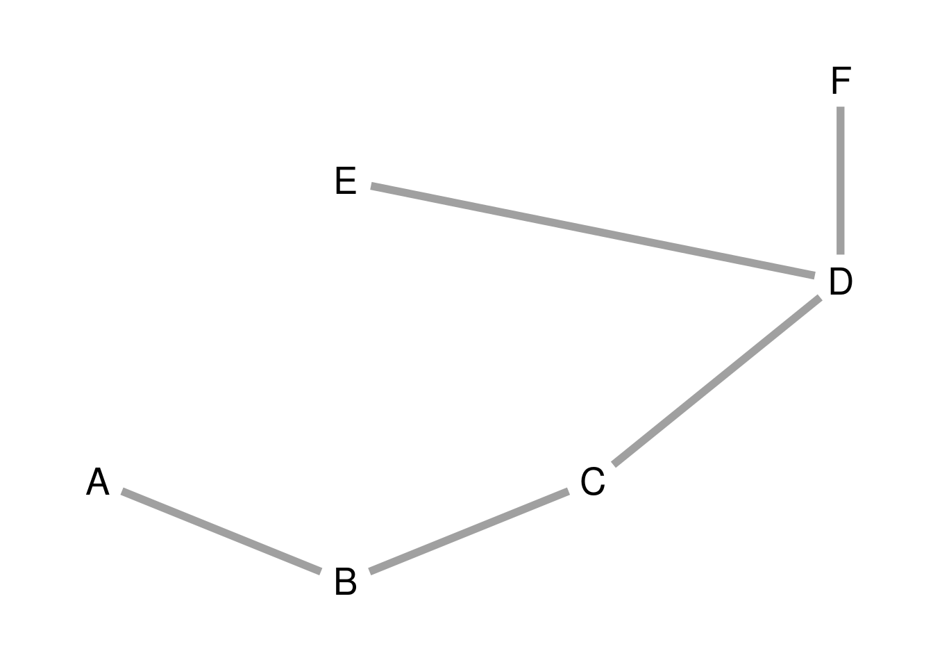
Session Info
## R version 4.4.0 (2024-04-24)
## Platform: x86_64-pc-linux-gnu
## Running under: Linux Mint 21.1
##
## Matrix products: default
## BLAS:   /usr/lib/x86_64-linux-gnu/blas/libblas.so.3.10.0
## LAPACK: /usr/lib/x86_64-linux-gnu/lapack/liblapack.so.3.10.0
##
## locale:
##  [1] LC_CTYPE=es_ES.UTF-8       LC_NUMERIC=C
##  [3] LC_TIME=es_ES.UTF-8        LC_COLLATE=es_ES.UTF-8
##  [5] LC_MONETARY=es_ES.UTF-8    LC_MESSAGES=es_ES.UTF-8
##  [7] LC_PAPER=es_ES.UTF-8       LC_NAME=C
##  [9] LC_ADDRESS=C               LC_TELEPHONE=C
## [11] LC_MEASUREMENT=es_ES.UTF-8 LC_IDENTIFICATION=C
##
## time zone: Europe/Madrid
## tzcode source: system (glibc)
##
## attached base packages:
## [1] stats     graphics  grDevices utils     datasets  methods   base
##
## other attached packages:
## [1] ggraph_2.2.1    ggplot2_3.5.1   tidygraph_1.3.1
##
## loaded via a namespace (and not attached):
##  [1] viridis_0.6.5      sass_0.4.9         utf8_1.2.4         generics_0.1.3
##  [5] tidyr_1.3.1        blogdown_1.19      digest_0.6.35      magrittr_2.0.3
##  [9] evaluate_0.23      grid_4.4.0         bookdown_0.39      fastmap_1.1.1
## [13] jsonlite_1.8.8     ggrepel_0.9.5      gridExtra_2.3      purrr_1.0.2
## [17] fansi_1.0.6        viridisLite_0.4.2  scales_1.3.0       tweenr_2.0.3
## [21] jquerylib_0.1.4    cli_3.6.2          graphlayouts_1.1.1 rlang_1.1.3
## [25] polyclip_1.10-6    munsell_0.5.1      withr_3.0.0        cachem_1.0.8
## [29] yaml_2.3.8         tools_4.4.0        memoise_2.0.1      dplyr_1.1.4
## [33] colorspace_2.1-0   vctrs_0.6.5        R6_2.5.1           lifecycle_1.0.4
## [37] MASS_7.3-60        pkgconfig_2.0.3    pillar_1.9.0       bslib_0.7.0
## [41] gtable_0.3.5       glue_1.7.0         Rcpp_1.0.12        ggforce_0.4.2
## [45] highr_0.10         xfun_0.43          tibble_3.2.1       tidyselect_1.2.1
## [49] rstudioapi_0.16.0  knitr_1.46         farver_2.1.1       htmltools_0.5.8.1
## [53] igraph_2.0.3       labeling_0.4.3     rmarkdown_2.26     compiler_4.4.0