In this post, I will make a short introduction to decision trees with the rpart package. This package implements the ideas about classification and regression trees presented in Breiman et al. (1983). I will present how rpart can be used for classification and numerical prediction, and how to plot the outcome of rpart using the rpart.plot package.
I will also use the dplyr and ggplot2 for data manipulation and visualization, BAdatasets to access the WineQuality dataset, mlbench to access the BostonHousing dataset and yardstick to obtain classification metrics.
library(dplyr)
library(ggplot2)
library(rpart)
library(rpart.plot)
library(BAdatasets)
library(mlbench)
library(yardstick)
Let’s start with the same set of synthetic data we used for C50:
n <- 400
set.seed(2020)
x <- c(runif(n*0.5, 0, 10), runif(n*0.25, 4, 10), runif(n*0.25, 0, 6))
y <- c(runif(n*0.5, 0, 5), runif(n*0.25, 4, 10), runif(n*0.25, 4, 10))
class <- as.factor(c(rep("a", n*0.5), c(rep("b", n*0.25)), c(rep("c", n*0.25))))

s_data <- tibble(x=x, y=y, class = class)
The rpart function uses the formula and data syntax. We can use rpart.plot to see the result:
dt01 <- rpart(class ~  ., s_data)
rpart.plot(dt01)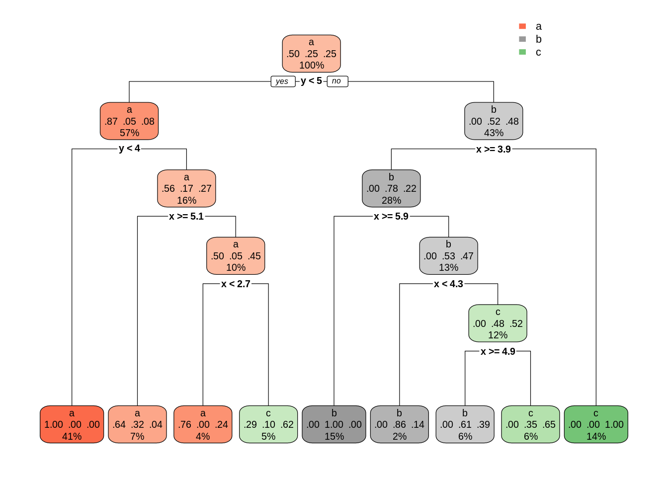
This classification is very precise and complex, but also prone to overfitting. We can control how precise and therefore prone to overfitting a rpart tree is with the complexity parameter cp. Any split that does not decrease the overall lack of fit by a factor of cp is not attempted. Small values of cp will create large trees and large values may not produce any tree. The default value of cp is of 0.01. Let’s see the result to increase cp by an order of magnitude:
dt02 <- rpart(class ~  ., s_data, cp = 0.1)
rpart.plot(dt02)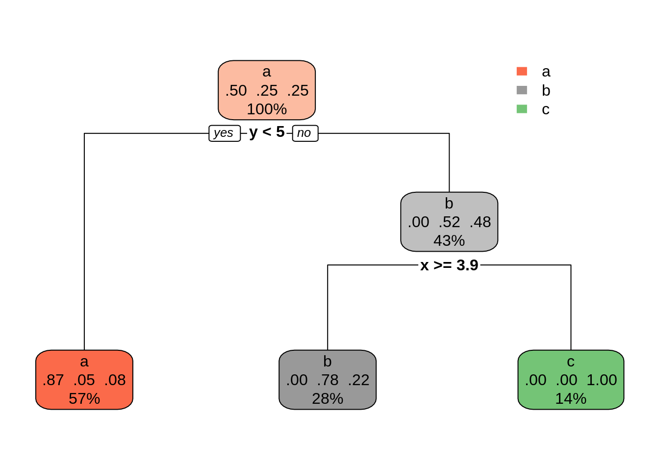
The outcome is similar to the obtained with C50 and can represent a good balance between bias and variance. Other ways of controlling tree size can be found at rpart.control.
Classifying with rpart
Let’s build the wines table of features predicting quality of red and white Portugese wines from data of WineQuality:
data("WineQuality")

red <- WineQuality$red %>%
  mutate(type = "red")
white <- WineQuality$white %>%
  mutate(type = "white")

wines <- bind_rows(red, white)
wines <- wines %>%
  mutate(quality = case_when(quality == 3 ~ 4,
                             quality == 9 ~ 8,
                             !quality %in% c(3,9) ~ quality))
wines <- wines %>%
  mutate(quality = factor(quality))
Let’s see the tree we obtain with rpart defaults:
dt_wines01 <- rpart(quality ~ ., wines)
rpart.plot(dt_wines01)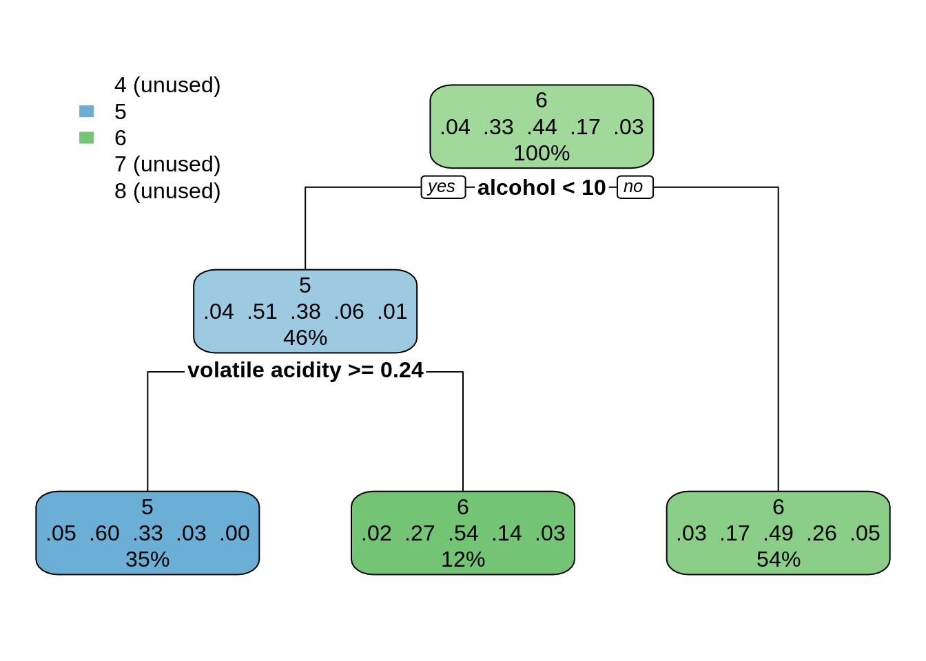
This classification looks too simplistic, as it has not been able to predict extreme values of quality. Let’s try a much smaller value of cp:
dt_wines02 <- rpart(quality ~ ., wines, cp = 0.0001)The resulting tree is too large to plot. Let’s use the predict function with type = "class" to obtain the predicted values for each element of the sample.
table_wines <- data.frame(value = wines$quality, pred = predict(dt_wines02, wines, type = "class"))Here is the confusion matrix:
conf_mat(table_wines, truth = value, estimate = pred)## Truth
## Prediction 4 5 6 7 8
## 4 59 29 23 10 0
## 5 103 1693 323 97 15
## 6 72 350 2332 275 60
## 7 11 58 143 685 59
## 8 1 8 15 12 64And here some classification metrics:
class_metrics <- metric_set(accuracy, precision, recall)
class_metrics(table_wines, truth = value, estimate = pred)
## # A tibble: 3 × 3
## .metric .estimator .estimate
## <chr> <chr> <dbl>
## 1 accuracy multiclass 0.744
## 2 precision macro 0.672
## 3 recall macro 0.562The classification metrics are not as good as with C50, as rpart does not implement winnowing and boosting. But maybe this classification is less prone to overfitting.
rpart offers a measure of variable importance equal to the sum of the goodness of split measures for each split for which it was the primary variable:
dt_wines02$variable.importance## alcohol density total sulfur dioxide
## 524.12183 495.09604 417.53959
## residual sugar chlorides volatile acidity
## 367.55782 344.47974 338.19316
## free sulfur dioxide fixed acidity pH
## 333.89703 270.91568 255.05421
## sulphates citric acid type
## 249.26864 242.07769 76.33693The variables used in early splits tend to have higher variable importance.
Prediction of house prices in Boston Housing with rpart
Let’s see now how can we use rpart for numerical prediction. I will be using the BostonHousing dataset presented by Harrison and Rubinfeld (1978). The target variable is medv, the median value of owner-occupied homes for each Boston census tract.
data("BostonHousing")
BostonHousing %>%
  glimpse()
## Rows: 506
## Columns: 14
## $ crim <dbl> 0.00632, 0.02731, 0.02729, 0.03237, 0.06905, 0.02985, 0.08829,…
## $ zn <dbl> 18.0, 0.0, 0.0, 0.0, 0.0, 0.0, 12.5, 12.5, 12.5, 12.5, 12.5, 1…
## $ indus <dbl> 2.31, 7.07, 7.07, 2.18, 2.18, 2.18, 7.87, 7.87, 7.87, 7.87, 7.…
## $ chas <fct> 0, 0, 0, 0, 0, 0, 0, 0, 0, 0, 0, 0, 0, 0, 0, 0, 0, 0, 0, 0, 0,…
## $ nox <dbl> 0.538, 0.469, 0.469, 0.458, 0.458, 0.458, 0.524, 0.524, 0.524,…
## $ rm <dbl> 6.575, 6.421, 7.185, 6.998, 7.147, 6.430, 6.012, 6.172, 5.631,…
## $ age <dbl> 65.2, 78.9, 61.1, 45.8, 54.2, 58.7, 66.6, 96.1, 100.0, 85.9, 9…
## $ dis <dbl> 4.0900, 4.9671, 4.9671, 6.0622, 6.0622, 6.0622, 5.5605, 5.9505…
## $ rad <dbl> 1, 2, 2, 3, 3, 3, 5, 5, 5, 5, 5, 5, 5, 4, 4, 4, 4, 4, 4, 4, 4,…
## $ tax <dbl> 296, 242, 242, 222, 222, 222, 311, 311, 311, 311, 311, 311, 31…
## $ ptratio <dbl> 15.3, 17.8, 17.8, 18.7, 18.7, 18.7, 15.2, 15.2, 15.2, 15.2, 15…
## $ b <dbl> 396.90, 396.90, 392.83, 394.63, 396.90, 394.12, 395.60, 396.90…
## $ lstat <dbl> 4.98, 9.14, 4.03, 2.94, 5.33, 5.21, 12.43, 19.15, 29.93, 17.10…
## $ medv <dbl> 24.0, 21.6, 34.7, 33.4, 36.2, 28.7, 22.9, 27.1, 16.5, 18.9, 15…The syntax for numerical prediction is similar to classification: rpart knows the type of problem by the class of target variable. The predicted value for the observations in a leaf is the average value of the target variable for the observations included in it.
dt_bh <- rpart(medv ~ ., BostonHousing)
rpart.plot(dt_bh)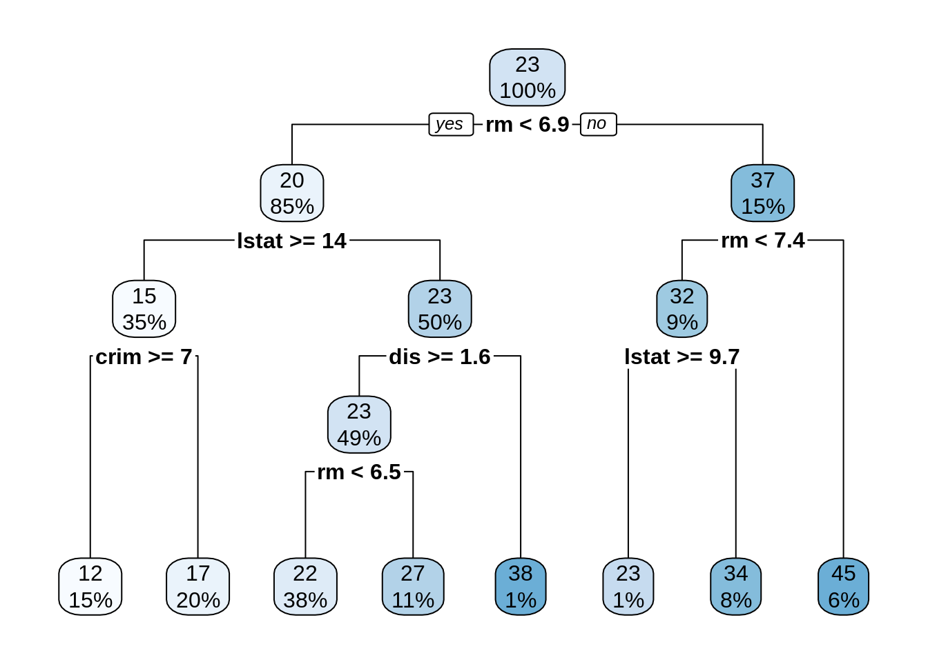
I have used the default cp = 0.01, obtaining a tree with a reasonable fit. Let’s examine variable importance:
dt_bh$variable.importance## rm lstat dis indus tax ptratio nox
## 23825.9224 15047.9426 5385.2076 5313.9748 4205.2067 4202.2984 4166.1230
## age crim zn rad b
## 3969.2913 2753.2843 1604.5566 1007.6588 408.1277To use the yardstick capabilities for numerical prediction, I am storing the real and predicted values of the target variable in a data frame.
table_bh <- data.frame(value = BostonHousing$medv,
                       pred = predict(dt_bh, BostonHousing))
Here I am obtaining the metrics, which show a reasonable fit.
np_metrics <- metric_set(rsq, rmse, mae)
np_metrics(table_bh, truth = value, estimate = pred)
## # A tibble: 3 × 3
## .metric .estimator .estimate
## <chr> <chr> <dbl>
## 1 rsq standard 0.808
## 2 rmse standard 4.03
## 3 mae standard 2.91Here is the plot of real versus predicted values. The algorithm provides as many predicted values as terminal nodes of the tree.
ggplot(table_bh, aes(value, pred)) +
  geom_point() +
  geom_abline(intercept = 0, slope = 1, color = "red") +
  theme_minimal() +
  labs(x = "real values", y = "predicted values", title = "Prediction of Boston Housing with rpart")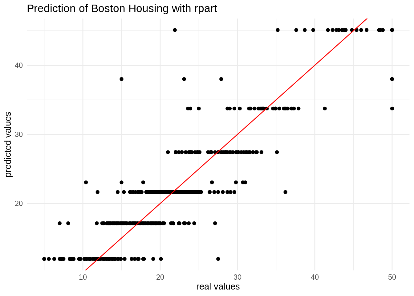
The rpart package implements in R the decision tree techniques presented in the CART book by Breiman et al. (1983). The package can be used for classification and numerical prediction. An effective implementation calls for tuning of some of the parameters of rpart.control, for instance the complexity parameter cp.
References
- BAdatasets web: https://github.com/jmsallan/BAdatasets
- Atkinson, E. J. The
rpartpackage. https://github.com/bethatkinson/rpart - Breiman, L., Friedman, J. H., Olshen, R. A., & Stone, C. J. (1983). Classification and regression trees. Wadsworth, Belmont, CA.
- Harrison, D. and Rubinfeld, D.L. (1978). Hedonic prices and the demand for clean air. Journal of Environmental Economics and Management, 5, 81–102.
- Milborrow, S. (2021). Plotting
rparttrees with therpart.plotpackage. http://www.milbo.org/rpart-plot/prp.pdf - Therneau, T. M.; Atkinson, E. J. (2022). An Introduction to Recursive Partitioning Using the RPART Routines. https://cran.r-project.org/web/packages/rpart/vignettes/longintro.pdf Mayo Foundation.
Session info
## R version 4.2.1 (2022-06-23)
## Platform: x86_64-pc-linux-gnu (64-bit)
## Running under: Linux Mint 19.2
##
## Matrix products: default
## BLAS:   /usr/lib/x86_64-linux-gnu/openblas/libblas.so.3
## LAPACK: /usr/lib/x86_64-linux-gnu/libopenblasp-r0.2.20.so
##
## locale:
##  [1] LC_CTYPE=es_ES.UTF-8       LC_NUMERIC=C
##  [3] LC_TIME=es_ES.UTF-8        LC_COLLATE=es_ES.UTF-8
##  [5] LC_MONETARY=es_ES.UTF-8    LC_MESSAGES=es_ES.UTF-8
##  [7] LC_PAPER=es_ES.UTF-8       LC_NAME=C
##  [9] LC_ADDRESS=C               LC_TELEPHONE=C
## [11] LC_MEASUREMENT=es_ES.UTF-8 LC_IDENTIFICATION=C
##
## attached base packages:
## [1] stats     graphics  grDevices utils     datasets  methods   base
##
## other attached packages:
## [1] yardstick_0.0.9  mlbench_2.1-3    BAdatasets_0.1.0 rpart.plot_3.1.0
## [5] rpart_4.1.16     ggplot2_3.3.5    dplyr_1.0.9
##
## loaded via a namespace (and not attached):
##  [1] Rcpp_1.0.8.3     highr_0.9        plyr_1.8.7       pillar_1.7.0
##  [5] bslib_0.3.1      compiler_4.2.1   jquerylib_0.1.4  tools_4.2.1
##  [9] digest_0.6.29    gtable_0.3.0     jsonlite_1.8.0   evaluate_0.15
## [13] lifecycle_1.0.1  tibble_3.1.6     pkgconfig_2.0.3  rlang_1.0.2
## [17] cli_3.3.0        DBI_1.1.2        rstudioapi_0.13  yaml_2.3.5
## [21] blogdown_1.9     xfun_0.30        fastmap_1.1.0    withr_2.5.0
## [25] stringr_1.4.0    knitr_1.39       pROC_1.18.0      generics_0.1.2
## [29] vctrs_0.4.1      sass_0.4.1       grid_4.2.1       tidyselect_1.1.2
## [33] glue_1.6.2       R6_2.5.1         fansi_1.0.3      rmarkdown_2.14
## [37] bookdown_0.26    farver_2.1.0     purrr_0.3.4      magrittr_2.0.3
## [41] scales_1.2.0     htmltools_0.5.2  ellipsis_0.3.2   assertthat_0.2.1
## [45] colorspace_2.0-3 labeling_0.4.2   utf8_1.2.2       stringi_1.7.6
## [49] munsell_0.5.0    crayon_1.5.1