Geographical coordinates

To plot airport networks, we need the latitude and longitude of airports. This information is stored in the Position node attribute. Dataset help tells us that this position is presented as “WGS coordinates”. After some research, we can learn that the position is in the latitude/longitude in the form PDDMMSS PDDDMMSS or PDDMMSS PDDMMSS, where P is the position of coordinates (N and S for latitude, E and W for longitude) and DD, MM and SS are the degrees, minutes and seconds, respectively.

The WGS_latlon function picks this format, and returns latitude and longitude values. Let’s apply it to airport coordinates.

WGS_latlon <- function(wgs){
  
  m <- str_split_fixed(wgs, " ", n = 2)
  pos <- str_sub(m, start = 1, end = 1)
  sign <- ifelse(pos %in% c("N", "E"), 1, -1)
  value <- matrix(str_sub(m, start = 2), ncol = 2)
  value <- ifelse(nchar(value) == 6, paste0("0", value), value)
  
  degree <- as.numeric(str_sub(value, start = 1, end = 3))
  minute <- as.numeric(str_sub(value, start = 4, end = 5))
  second <- as.numeric(str_sub(value, start = 6, end = 7))
  
  dms <- degree + minute/60 + second/3600
  dms <- dms * sign
  dms <- matrix(dms, ncol = 2)
  
  return(dms)
}


coords <- WGS_latlon (US_airports %>%
                        activate(nodes) %>%
                        pull(Position))

## Warning in WGS_latlon(US_airports %>% activate(nodes) %>% pull(Position)): NAs
## introducidos por coerción

## Warning in WGS_latlon(US_airports %>% activate(nodes) %>% pull(Position)): NAs
## introducidos por coerción

I have obtained a NAs introduced by coercion warning, meaning that probably there are some missing data. Let’s load the function outcome as node attributes first:

US_airports <- US_airports %>%
  activate(nodes) %>%
  mutate(lat = coords[ , 1],
         lon = coords[, 2])

Now we can examine the missing data:

US_airports %>%
  activate(nodes) %>%
  filter(is.na(lat), is.na(lon))

## # A tbl_graph: 1 nodes and 0 edges
## #
## # A rooted tree
## #
## # Node Data: 1 × 5 (active)
##   name  City          Position   lat   lon
##   <chr> <chr>         <chr>    <dbl> <dbl>
## 1 KTN   Ketchikan, AK MIAMI       NA    NA
## #
## # Edge Data: 0 × 8
## # … with 8 variables: from <int>, to <int>, Carrier <chr>, Departures <dbl>,
## #   Seats <dbl>, Passengers <dbl>, Aircraft <int>, Distance <dbl>

KTN happens to be the Ketchikan International Airport. I have retrieved its coordinates from Wikipedia and added them to the dataset:

lat_KTN <- 55 + 21/60 + 15/3600
lon_KTN <- - (131 + 42/60 + 40/3600)

US_airports <- US_airports %>%
  activate(nodes) %>%
  mutate(lat = replace(lat, is.na(lat), lat_KTN),
         lon = replace(lon, is.na(lon), lon_KTN))

US_airports %>%
  activate(nodes) %>%
  filter(name == "KTN")

## # A tbl_graph: 1 nodes and 0 edges
## #
## # A rooted tree
## #
## # Node Data: 1 × 5 (active)
##   name  City          Position   lat   lon
##   <chr> <chr>         <chr>    <dbl> <dbl>
## 1 KTN   Ketchikan, AK MIAMI     55.4 -132.
## #
## # Edge Data: 0 × 8
## # … with 8 variables: from <int>, to <int>, Carrier <chr>, Departures <dbl>,
## #   Seats <dbl>, Passengers <dbl>, Aircraft <int>, Distance <dbl>

Obtaining airline airport networks

Now I am interested in obtaining the airport networks of selected carriers. The carrier_network function picks the nodes and edges of a carrier to build an airline airport network in the following way:

• Selects the edges associated to a carrier filtering by the value of Carrier in the edge table.
• To obtain airport nodes, it calculates node degree with centrality_degree. Node degree is the sum of edges arriving or departing from the node. So the function retains only nodes with degree different from zero. Finally, the function removes node degree.

carrier_network <- function(carrier){
  g <- US_airports %>%
          activate(edges) %>%
          filter(Carrier == carrier) %>%
          activate(nodes) %>%
          mutate(deg = centrality_degree()) %>%
          filter(deg != 0)
  
  g <- g %>%
    activate(nodes) %>%
    select(-deg)
  
  return(g)
}

Let’s obtain the airport networks of Southwest Airlines, Delta Air Lines and Hageland Aviation Service:

WN_airports <- carrier_network("Southwest Airlines Co.")
DL_airports <- carrier_network("Delta Air Lines Inc.")
H6_airports <- carrier_network("Hageland Aviation Service")

Plotting airline airport networks

The function carrier_graph plots the graph of an airport network obtained from US_airports. It uses ggraph to plot the network, using as layout (position of nodes) the latitude and longitude of each airport. Airline airport networks can be considered spatial networks, so I have overlaid a map with geom_sf. The fill of the map needs a value of alpha transparency smaller than one to see the network over the map. Node size is proportional to betweenness, so hub airports are presented with dots of larger size. The alaska logical variable allows focusing the map on Alaska, and us on mainland of the United States.

carrier_graph <- function(carrier_network, us = TRUE, alaska = TRUE){
  
  carrier_network <- carrier_network %>%
    activate(nodes) %>%
    mutate(btw = centrality_betweenness())
  
  #finding map
  us_map <- WorldMap1_10
  
  #position of airports
  layout <- as.matrix(carrier_network %>%
                        activate(nodes) %>%
                        as_tibble() %>%
                        select(lon, lat), byrow = TRUE)
  
  #finding hubs
  
  plot <- ggraph(carrier_network, layout = layout) +
    geom_edge_link(width = 0.1) +
    geom_node_point(color = "#CC0000", aes(size = btw)) +
    geom_sf(data = us_map, alpha = 0.25, fill = "#994C00") +
    # theme_void() +
    theme(panel.background = element_rect(fill = "#CCE5FF"), 
          legend.position = "none")
  
  if(alaska == TRUE & us == FALSE){
    plot <- plot +
      coord_sf(xlim = c(-180, -125), ylim = c(50, 71))
  }
  
  if(alaska == TRUE & us == TRUE){
    plot <- plot +
      coord_sf(xlim = c(-180, -62), ylim = c(17 , 71))
  }
  
  if(alaska == FALSE & us == TRUE){
    plot <- plot +
      coord_sf(xlim = c(-130, -62), ylim = c(25, 50))
  }
  
  return(plot)
}

Let’s apply the carrier_graph function to each of the airlines.

carrier_graph(WN_airports, alaska = FALSE)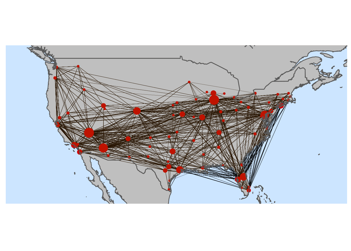

Southwest Airlines network is dense, with many airports with a similar value of betweenness. This is typical of a point-to-point route network. This route network is typical of low cost carriers.

carrier_graph(DL_airports)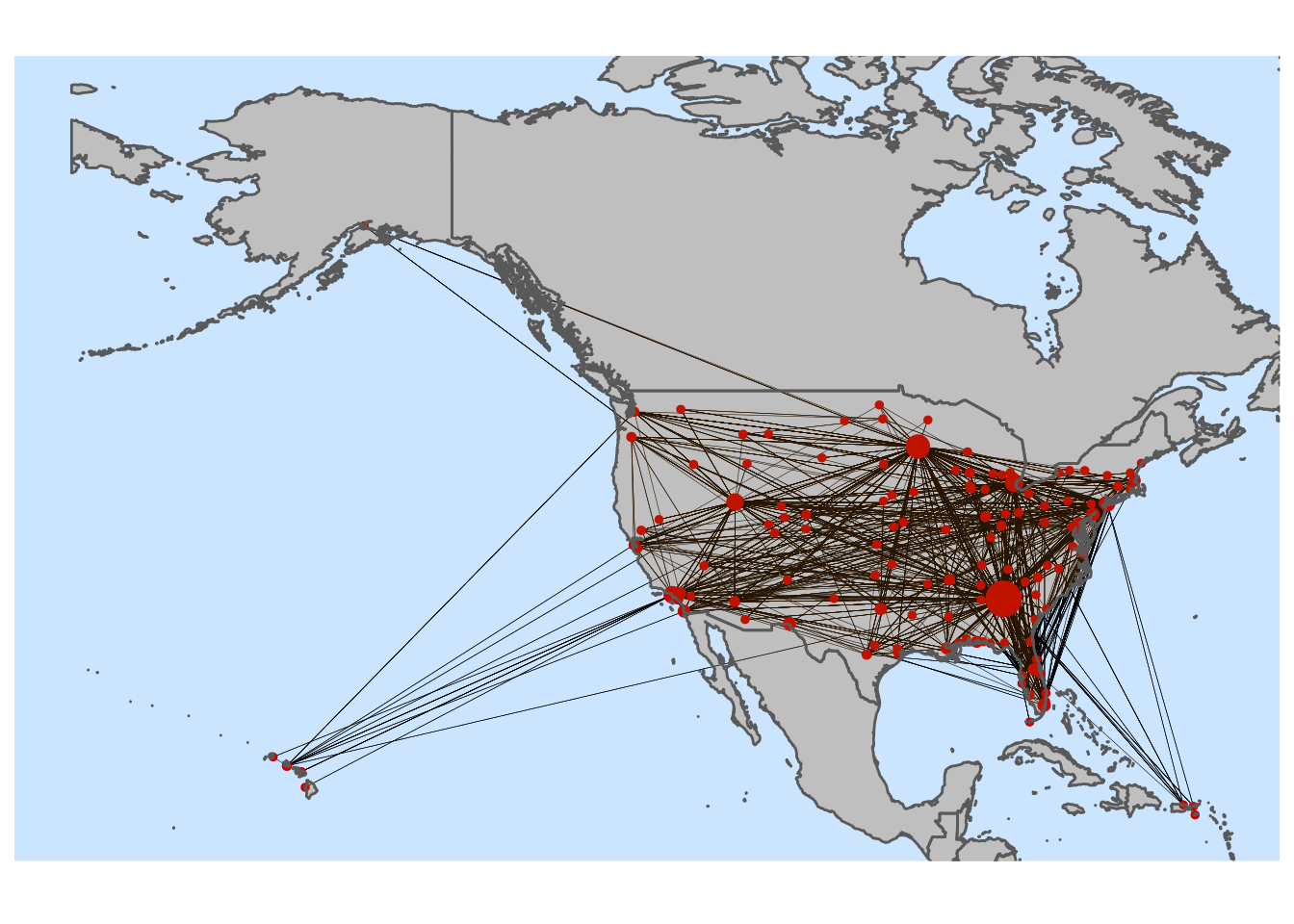

The graph of Delta Air Lines is very dense, covering a large range of airports. The difference of size between nodes is large, meaning that the operations of the airline are centered in their hubs, which are the Atlanta ATL and Minneapolis MSP airports. Delta Airlines is adopting a hub-and-spoke route network, with several hubs for domestic US flights. This network is typical of full service carriers.

carrier_graph(H6_airports, us = FALSE)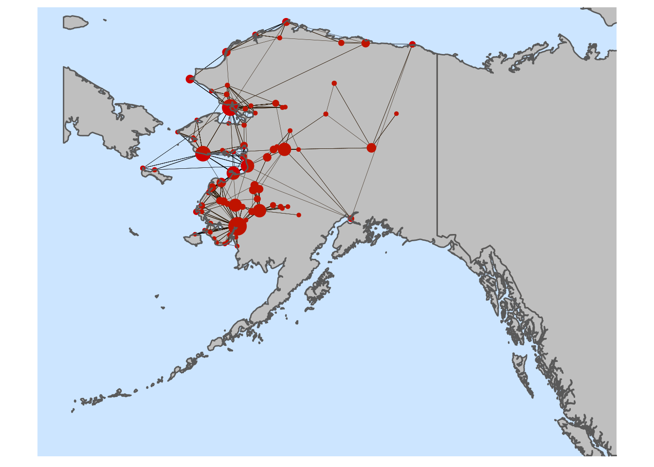

Hageland Aviation Services was a regional Alaskan airline, covering mainly Alaskan routes, which ceased operations in 2019. The Alaskan airport network is quite dense, as many towns have no roads leading to them, and are only accessible by airplane or by ship, as they have no roads connecting them to the rest of America. This regional airline had no large hub, so it has a point to point route network.

References

• Lordan, O., Sallan, J. M., Escorihuela, N., & Gonzalez-Prieto, D. (2016). Robustness of airline route networks. Physica A: Statistical Mechanics and its Applications, 445, 18-26. https://doi.org/10.1016/j.physa.2015.10.053
• Pedersen, T. L. (2017). Introducing tidygraph. https://www.data-imaginist.com/2017/introducing-tidygraph/
• Wikipedia. Ketchikan International Airport https://en.wikipedia.org/wiki/Ketchikan_International_Airport. Accessed 2021-11-28.
• Wikipedia. List of airports in Alaska. https://en.wikipedia.org/wiki/List_of_airports_in_Alaska. Accessed 2021-11-28.

Session info

## R version 4.1.2 (2021-11-01)
## Platform: x86_64-pc-linux-gnu (64-bit)
## Running under: Debian GNU/Linux 10 (buster)
## 
## Matrix products: default
## BLAS:   /usr/lib/x86_64-linux-gnu/blas/libblas.so.3.8.0
## LAPACK: /usr/lib/x86_64-linux-gnu/lapack/liblapack.so.3.8.0
## 
## locale:
##  [1] LC_CTYPE=es_ES.UTF-8       LC_NUMERIC=C              
##  [3] LC_TIME=es_ES.UTF-8        LC_COLLATE=es_ES.UTF-8    
##  [5] LC_MONETARY=es_ES.UTF-8    LC_MESSAGES=es_ES.UTF-8   
##  [7] LC_PAPER=es_ES.UTF-8       LC_NAME=C                 
##  [9] LC_ADDRESS=C               LC_TELEPHONE=C            
## [11] LC_MEASUREMENT=es_ES.UTF-8 LC_IDENTIFICATION=C       
## 
## attached base packages:
## [1] stats     graphics  grDevices utils     datasets  methods   base     
## 
## other attached packages:
## [1] tidygraph_1.2.0         ggraph_2.0.5            ggplot2_3.3.5          
## [4] BAdatasetsSpatial_0.1.0 sf_1.0-2                igraphdata_1.0.1       
## [7] stringr_1.4.0           dplyr_1.0.7            
## 
## loaded via a namespace (and not attached):
##  [1] tidyselect_1.1.1   xfun_0.23          bslib_0.2.5.1      graphlayouts_0.7.2
##  [5] purrr_0.3.4        colorspace_2.0-1   vctrs_0.3.8        generics_0.1.0    
##  [9] viridisLite_0.4.0  htmltools_0.5.1.1  s2_1.0.6           yaml_2.2.1        
## [13] utf8_1.2.1         rlang_0.4.12       e1071_1.7-8        jquerylib_0.1.4   
## [17] pillar_1.6.4       glue_1.4.2         withr_2.4.2        DBI_1.1.1         
## [21] tweenr_1.0.2       wk_0.5.0           lifecycle_1.0.0    munsell_0.5.0     
## [25] blogdown_1.5       gtable_0.3.0       evaluate_0.14      knitr_1.33        
## [29] class_7.3-19       fansi_0.5.0        highr_0.9          Rcpp_1.0.6        
## [33] KernSmooth_2.23-20 scales_1.1.1       classInt_0.4-3     jsonlite_1.7.2    
## [37] farver_2.1.0       gridExtra_2.3      ggforce_0.3.3      digest_0.6.27     
## [41] stringi_1.7.3      ggrepel_0.9.1      bookdown_0.24      polyclip_1.10-0   
## [45] grid_4.1.2         cli_3.0.1          tools_4.1.2        magrittr_2.0.1    
## [49] sass_0.4.0         proxy_0.4-26       tibble_3.1.5       crayon_1.4.1      
## [53] tidyr_1.1.4        pkgconfig_2.0.3    ellipsis_0.3.2     MASS_7.3-54       
## [57] rstudioapi_0.13    viridis_0.6.1      assertthat_0.2.1   rmarkdown_2.9     
## [61] R6_2.5.0           units_0.7-2        igraph_1.2.6       compiler_4.1.2