In this post, I will present how to plot complex variable functions. To do so, I will plot the gamma function, as it allows illustrating how to plot asymptotic functions. I will plot the function in its real domain first, and then produce 2D and 3D plots of the complex domain. I will use ggplot2 for two dimensional plots, and plotly for the 3D surface plot. To calculate the gamma function for complex numbers with imaginary component I will use the pracma package.
library(tidyverse)
library(pracma)
library(plotly)
The gamma function is defined for any complex number \(z\) as:
\[ \Gamma \left(z\right) = \int_0^\infty t^{z-1}e^{-t} dt \]
For every positive integer we have:
\[ \Gamma \left(n\right) = \left(n-1\right)! \]
That’s why the gamma function is considered as a one of the possible extensions of the factorial for complex numbers.
We can plot any function straight away with ggplot using the stat_function geom. Let’s see a straight away example:
ggplot() +
  stat_function(fun = \(x) x^2,
                xlim = c(-2, 2)) +
  theme_minimal()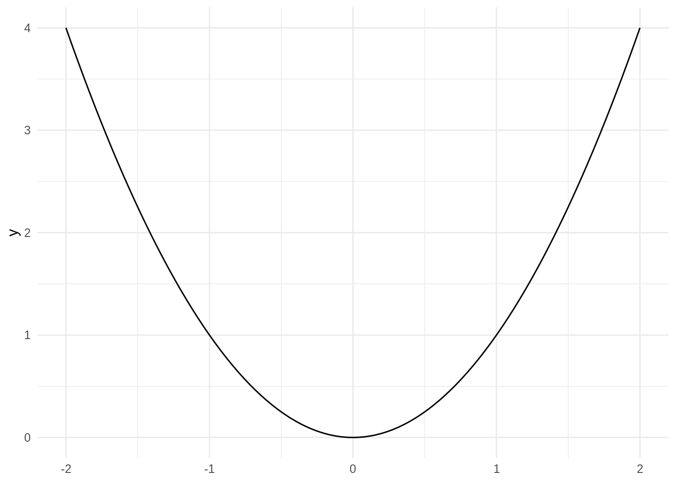
In stat_function, the function to plot is entered in fun, and the function domain to plot as xlim.
The gamma function for real values
Let’s do something similar with the gamma function, using the R base function gamma, for a range of positive and negative numbers. Here I am adding more arguments to stat_function:
n, the number of points to use to draw the curve.sizefor line width.
I have also added a scale_x_continuous to define the breaks of the x axis.
ggplot() +
  stat_function(fun = gamma,
                xlim = c(-7, 7),
                n = 1001,
                size = 1.2) +
  scale_x_continuous(breaks = -4:2) +
  theme_minimal()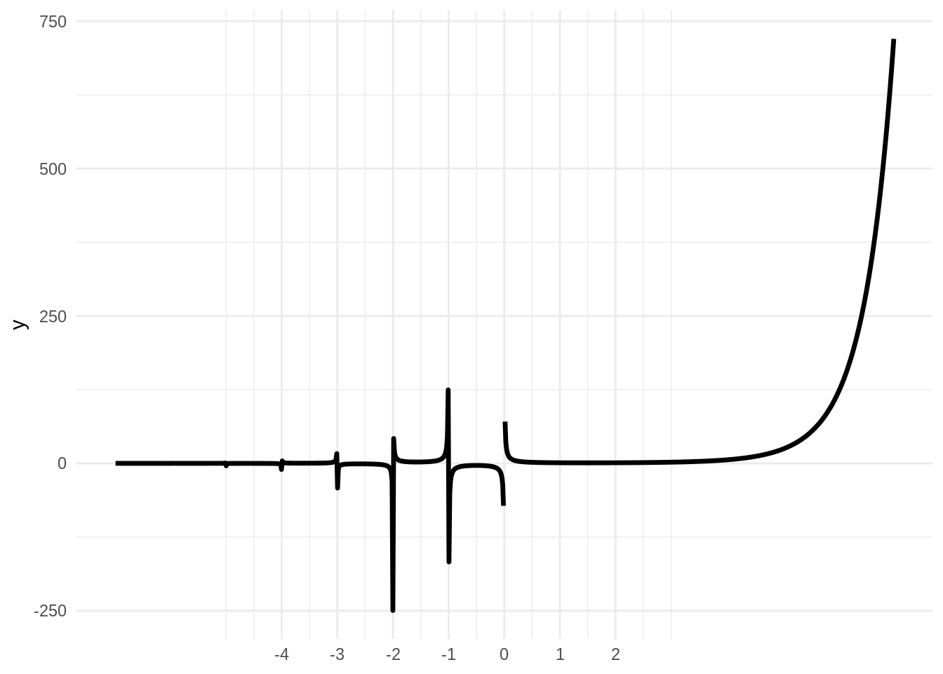
The resulting plot is not satisfactory, as the behavior for non-negative numbers is quite different from the rest of the domain. There seems to be vertical asymptotes for nonpositive integer numbers, and the function grows factorially for positive values. Therefore, I have opted to present two plots for the gamma function:
- a plot for positive real values, showing the relationship between gamma and factorial.
- a plot for non-positive real values, showing the asymptotic behaviour of the function.
This is the plot for positive values:
df1 <- tibble(x = 1:8,
             y = factorial(x-1))

ggplot(df1, aes(x, y)) +
  geom_point(size = 2) +
  stat_function(fun = gamma, size = 0.8, color = "#A0A0A0") +
  theme_minimal() +
  scale_x_continuous(breaks = 1:8) +
  ggtitle("gamma function (positive values)")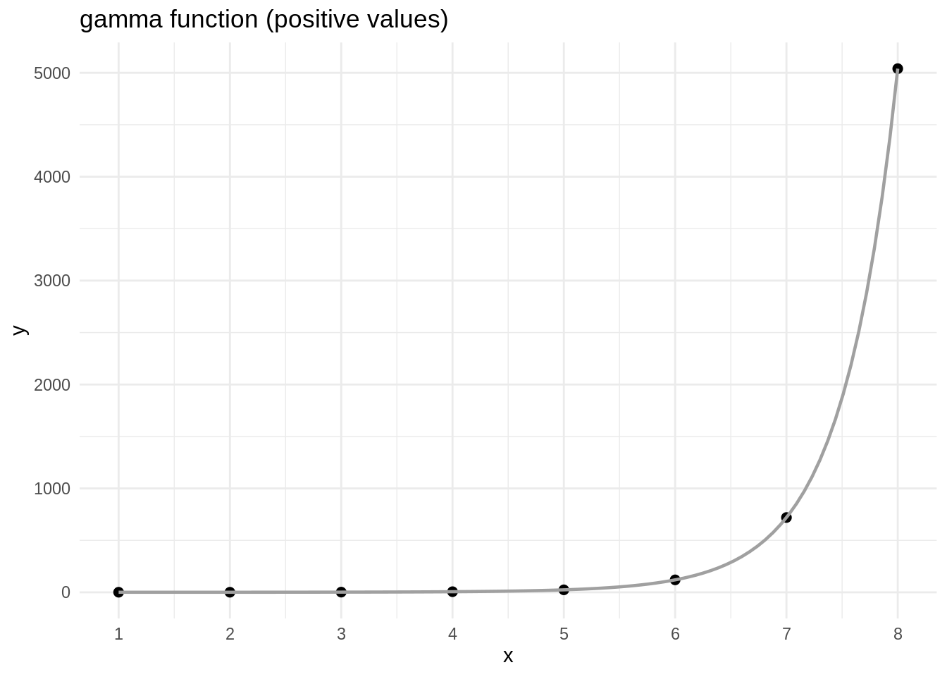
The dots in the plot represent \(\left(n-1\right)!\) for integer values. Its values come from table df1, and are plotted with geom_point. The gamma function is plotted with stat_function, adding a color argument. I have also added a title with ggtitle.
This is the plot for non-positive values.
df2 <- tibble(x = seq(-4, 2, length.out = 1000),
             y = gamma(x)) %>%
  mutate(y = ifelse(abs(y) < 20, y, NA))

ggplot(df2, aes(x, y)) +
  geom_line(size = 1.2) +
  geom_vline(xintercept = -4:0, size = 0.5, linetype = "dashed") +
  scale_x_continuous(breaks = -4:2) +
  theme_minimal() +
  ggtitle("gamma function (negative values)")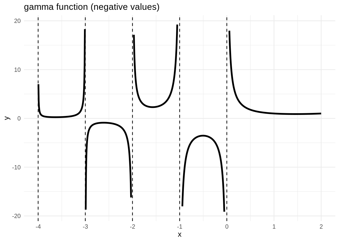
For the negative values, I do not use stat_function. Instead I defining values for the two axis in the df2 table. When the absolute value of the function is greater than 20 I turn it no NA, so the geom_line is interrupted. Finally, I am adding asymptotes for non-positive integers using geom_vline. Note that the value of xintercept is a vector, so all asymptotes are plotted in a single instruction.
The gamma function for complex values
Let’s see now how we can learn how is behaving the gamma function for the whole complex domain, including values with nonzero imaginary component. R has a cplx class for complex numbers, with real and imaginary components. The polar components can be obtained with the Mod and Arg functions.
The gamma function for the whole complex domain can be obtained with the gammaz function of the pracma package. To represent the function graphically, I have chosen to assign the real and imaginary component to axis x and y, and the module of the gamma function to axis z. I nave used the expand_grid function to define a grid of points, so we have 10,000 points in a 100x100 grid.
values <- expand_grid(r = seq(-2.5, 2.5, length.out = 100),
                      i = seq(-2.5, 2.5, length.out = 100)) %>%
  mutate(z = complex(real = r, imaginary = i),
         gamma = gammaz(z),
         mod = Mod(gamma),
         mod = ifelse(mod < 10, mod, 10))
We have two possibilities to represent a 3D function in 2D:
- Countour lines: we can do that with the
geom_contour()with the function values in azargument inaes. - Heatmap: heatmaps are plot with
geom_tile()with the function value in thefillargument inaes.
This plot presents a contour and a heatmap. I am plotting the tiles before the contour to present both, and I have added also a alpha value in the tile plot.
ggplot(values, aes(r, i)) +
  geom_tile(aes(fill = mod), alpha = 0.5) +
  scale_fill_gradient(name = "z",
                      low = "#FFFFCC",
                      high = "#FF0000") +
  geom_contour(aes(z = mod), color = "black", bins = 50) +
  theme_minimal()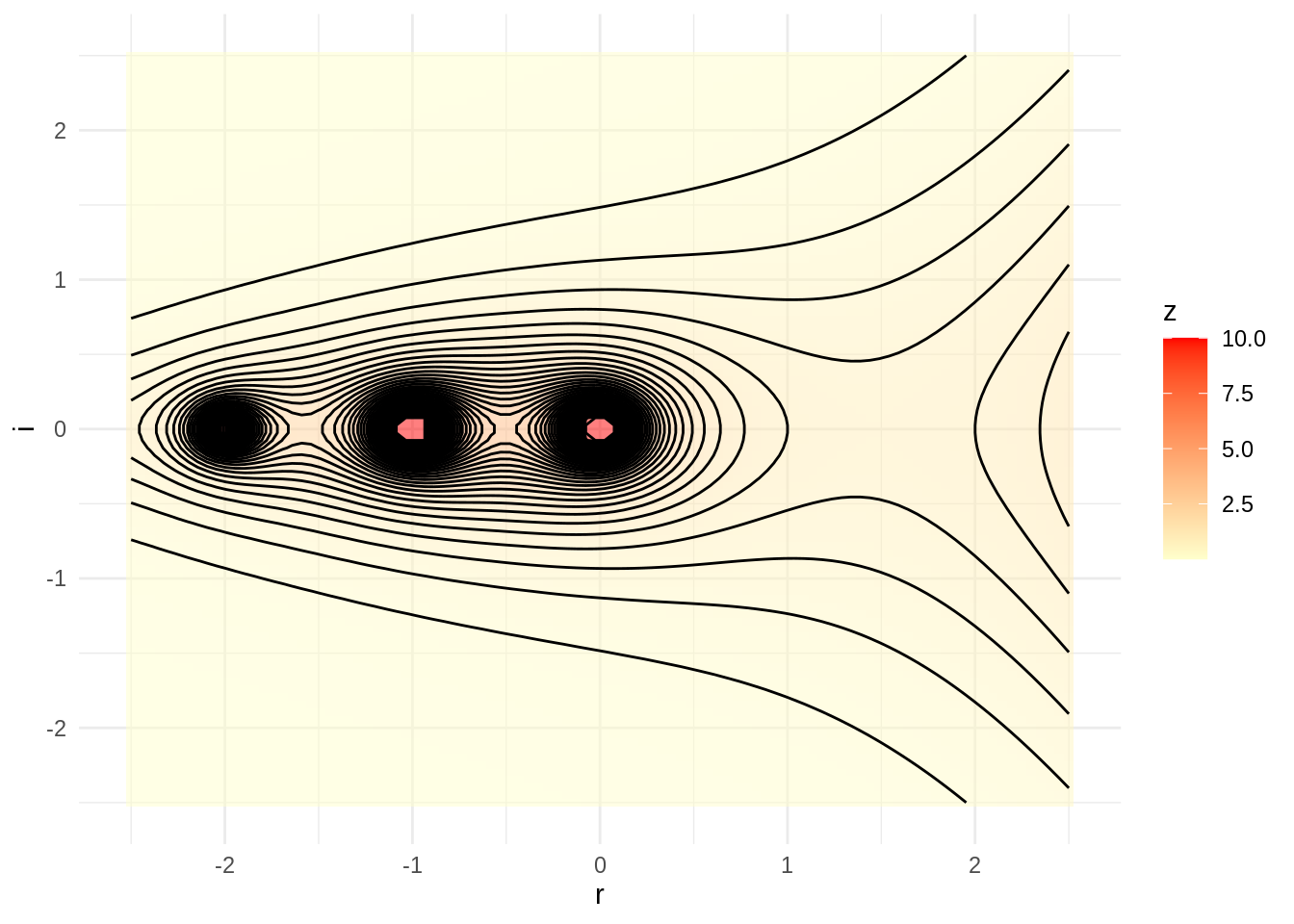
In the plot appear asymptotes in the integer negative values of the real axis.
To present a real 3D plot, the best option is to generate a surface in plotly.
n <- 100

x <- seq(-2.5, 2.5, length.out = n)
y <- seq(-3.5, 2.5, length.out = n)

t <- expand.grid(x = x, y = y)

t$mod <- Mod(gammaz(complex(real = t$x, imaginary = t$y)))
t$mod <- ifelse(t$mod < 5, t$mod, 5)

z <- matrix(t$mod, n, n)

plot_ly(x = x,
        y = y,
        z = z) |>
  layout(scene = list(xaxis = list(title = "r"),
                      yaxis = list(title = "i"),
                      zaxis = list(title = "mod"))) |>
  add_surface(colorscale = "Reds")
Session info
## R version 4.2.1 (2022-06-23)
## Platform: x86_64-pc-linux-gnu (64-bit)
## Running under: Linux Mint 19.2
##
## Matrix products: default
## BLAS:   /usr/lib/x86_64-linux-gnu/openblas/libblas.so.3
## LAPACK: /usr/lib/x86_64-linux-gnu/libopenblasp-r0.2.20.so
##
## locale:
##  [1] LC_CTYPE=es_ES.UTF-8       LC_NUMERIC=C
##  [3] LC_TIME=es_ES.UTF-8        LC_COLLATE=es_ES.UTF-8
##  [5] LC_MONETARY=es_ES.UTF-8    LC_MESSAGES=es_ES.UTF-8
##  [7] LC_PAPER=es_ES.UTF-8       LC_NAME=C
##  [9] LC_ADDRESS=C               LC_TELEPHONE=C
## [11] LC_MEASUREMENT=es_ES.UTF-8 LC_IDENTIFICATION=C
##
## attached base packages:
## [1] stats     graphics  grDevices utils     datasets  methods   base
##
## other attached packages:
##  [1] plotly_4.10.0   pracma_2.4.2    forcats_0.5.2   stringr_1.4.1
##  [5] dplyr_1.0.10    purrr_0.3.5     readr_2.1.3     tidyr_1.2.1
##  [9] tibble_3.1.8    ggplot2_3.3.6   tidyverse_1.3.1
##
## loaded via a namespace (and not attached):
##  [1] lubridate_1.8.0   assertthat_0.2.1  digest_0.6.30     utf8_1.2.2
##  [5] R6_2.5.1          cellranger_1.1.0  backports_1.4.1   reprex_2.0.2
##  [9] evaluate_0.17     highr_0.9         httr_1.4.4        blogdown_1.9
## [13] pillar_1.8.1      rlang_1.0.6       lazyeval_0.2.2    readxl_1.4.1
## [17] rstudioapi_0.13   data.table_1.14.2 jquerylib_0.1.4   rmarkdown_2.14
## [21] labeling_0.4.2    htmlwidgets_1.5.4 munsell_0.5.0     broom_1.0.1
## [25] compiler_4.2.1    modelr_0.1.9      xfun_0.34         pkgconfig_2.0.3
## [29] htmltools_0.5.3   tidyselect_1.1.2  bookdown_0.26     viridisLite_0.4.1
## [33] fansi_1.0.3       crayon_1.5.2      tzdb_0.3.0        dbplyr_2.2.1
## [37] withr_2.5.0       grid_4.2.1        jsonlite_1.8.3    gtable_0.3.0
## [41] lifecycle_1.0.3   DBI_1.1.2         magrittr_2.0.3    scales_1.2.1
## [45] cli_3.4.1         stringi_1.7.8     farver_2.1.1      fs_1.5.2
## [49] xml2_1.3.3        bslib_0.3.1       ellipsis_0.3.2    generics_0.1.2
## [53] vctrs_0.5.0       tools_4.2.1       glue_1.6.2        crosstalk_1.2.0
## [57] hms_1.1.2         fastmap_1.1.0     yaml_2.3.6        colorspace_2.0-3
## [61] isoband_0.2.5     rvest_1.0.3       knitr_1.40        haven_2.5.1
## [65] sass_0.4.1