In this post, I will present the workflow to create an horizontal barchart presenting a set of values. A good practice for those tables is to arrange bars in decreasing order of the value. We’ll see that we can to that with the fct_reorder function of forcats, included in the tidyverse.

I will be using the txhousing dataset, included in tidyverse, so I don’t need more than that:

library(tidyverse)

Let’s see which cities of Texas have the most expensive housing. For each city, I am computing a price variable, equal to the median of median prices from 2010 onwards:

txhousing |>
  filter(year >= 2010) |>
  group_by(city) |>
  summarise(price = median(median, na.rm = TRUE)) |>
  arrange(-price)

## # A tibble: 46 × 2
##    city                price
##    <chr>               <dbl>
##  1 Collin County      223100
##  2 Midland            212000
##  3 Austin             210200
##  4 Fort Bend          209800
##  5 Montgomery County  197100
##  6 NE Tarrant County  180000
##  7 South Padre Island 180000
##  8 Galveston          178600
##  9 Denton County      175300
## 10 Dallas             174200
## # … with 36 more rows

Let’s see the default plot of those values with geom_bar(stat = "identity"):

txhousing |>
  filter(year >= 2010) |>
  group_by(city) |>
  summarise(price = median(median, na.rm = TRUE)) |>
  ggplot(aes(city, price)) +
  geom_bar(stat = "identity")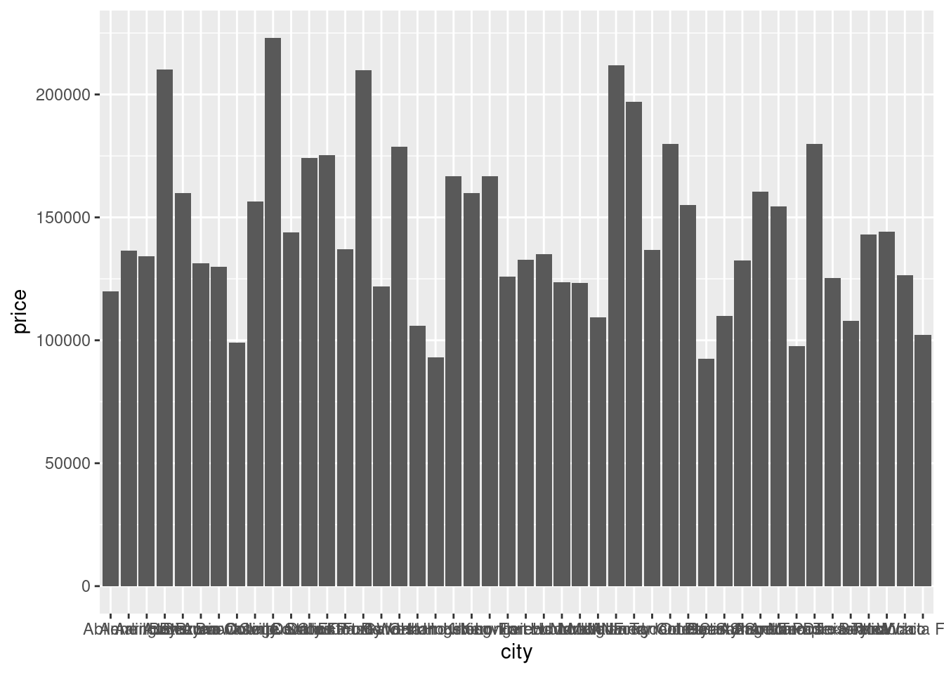

This plot is not nice, for several reasons:

• We cannot see the city names in the x axis.
• Bars are not arranged, so it is hard to see what are the most expensive cities.
• There are too many bars to see, which add little information if we focus on the more expensive cities.
• The standard output of ggplot has a lot of clutter.

We can get to see city names reversing axis. That’s why we present an horizontal bar chart:

txhousing |>
  filter(year >= 2010) |>
  group_by(city) |>
  summarise(price = median(median, na.rm = TRUE)) |>
  ggplot(aes(price, city)) +
  geom_bar(stat = "identity")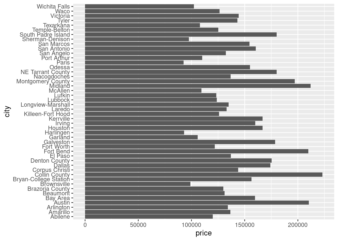

To reorder the cities, we use fct_reorder to change the city factor variable, so it is reordered by price:

txhousing |>
  filter(year >= 2010) |>
  group_by(city) |>
  summarise(price = median(median, na.rm = TRUE)) |>
  mutate(city = fct_reorder(city, price)) |>
  ggplot(aes(price, city)) +
  geom_bar(stat = "identity")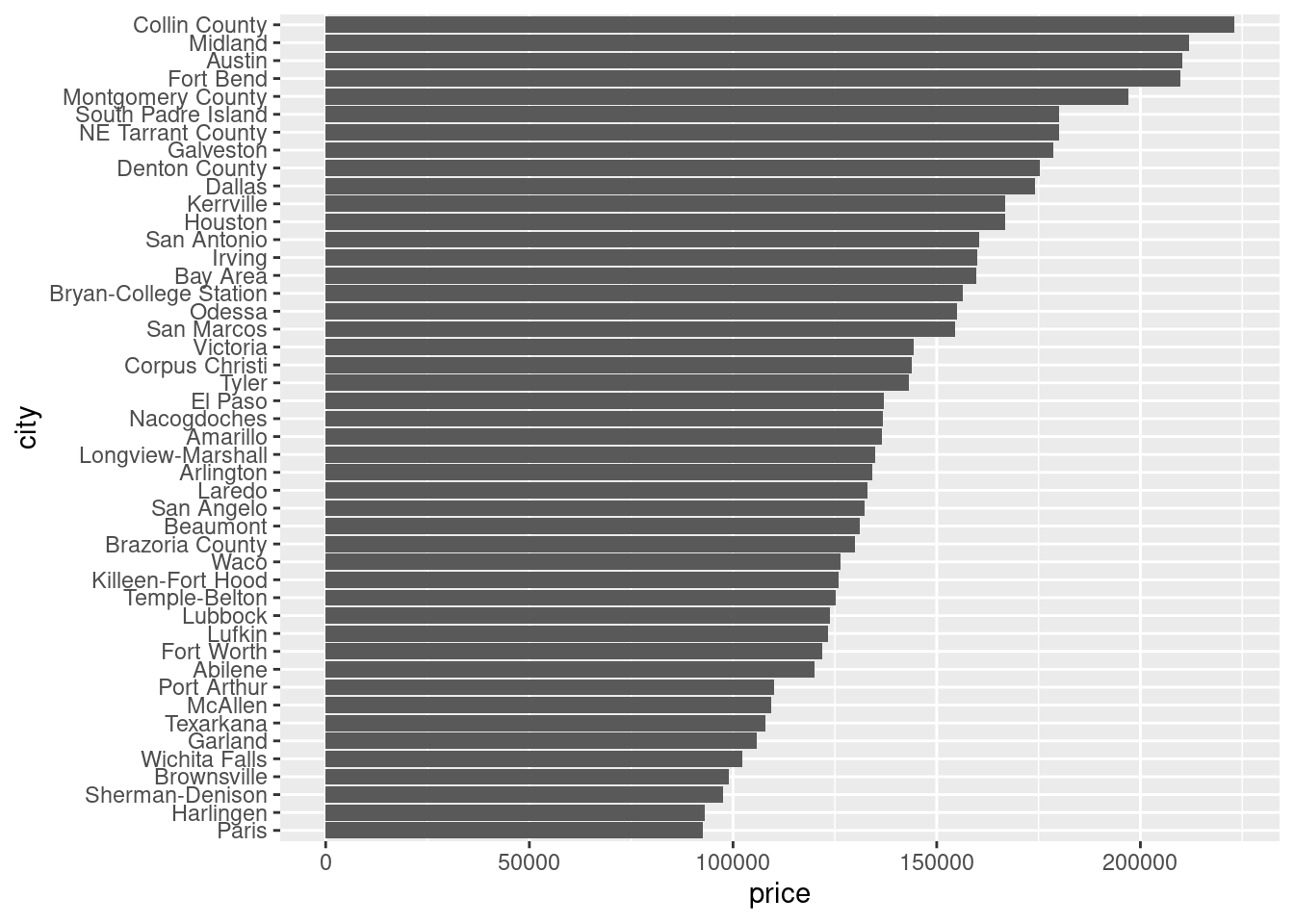

If we want to pick the ten largest cities instead of all cities, we need to arrange the table by price, and then slice it to pick the first ten rows. Note that fct_reorder reorders the chart, but not the table!

txhousing |>
  filter(year >= 2010) |>
  group_by(city) |>
  summarise(price = median(median, na.rm = TRUE)) |>
  arrange(-price) |>
  slice(1:10) |>
  mutate(city = fct_reorder(city, price)) |>
  ggplot(aes(price, city)) +
  geom_bar(stat = "identity")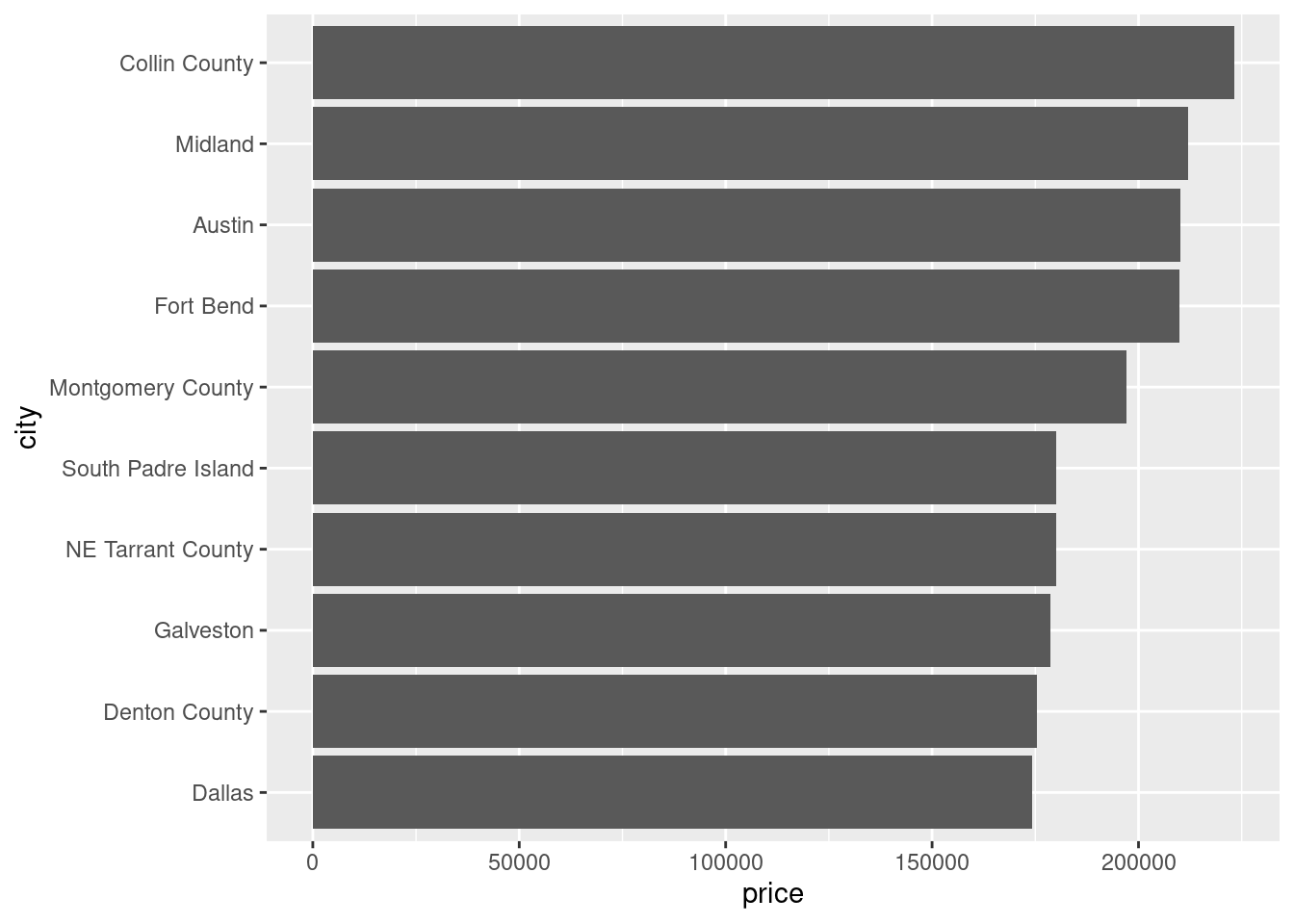

Finally, we can improve the look of the table by:

• setting a blue color for bars with fill parameter in geom_bar.
• removing the backgroun and axis with theme_minimal.
• change the size of the title and axis text with theme.
• adding a descriptive enough title and removing axis labels with labs.

txhousing |>
  filter(year >= 2010) |>
  group_by(city) |>
  summarise(price = median(median, na.rm = TRUE)) |>
  arrange(-price) |>
  slice(1:10) |>
  mutate(city = fct_reorder(city, price)) |>
  ggplot(aes(price, city)) +
  geom_bar(stat = "identity", fill = "#66B2FF") +
  theme_minimal() +
  theme(axis.text.y = element_text(size = 12),
        plot.title = element_text(size=15)) +
  labs(title = "The most expensive cities in Texas (median prices)", x = NULL, y = NULL)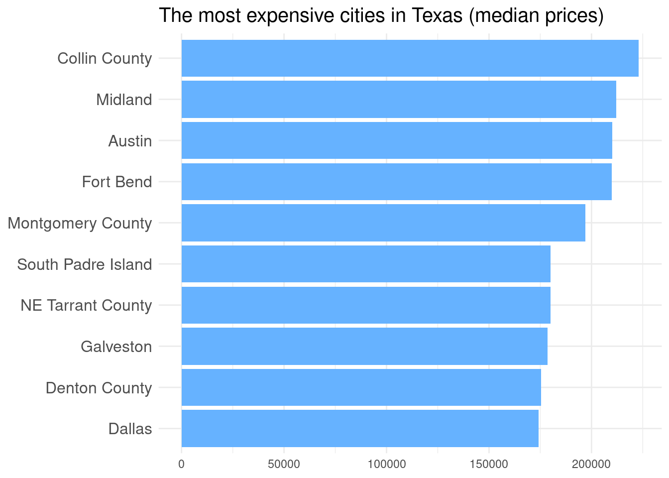

The resulting chart is hopefully easier to read and to interpret than the default one.

## R version 4.2.2 Patched (2022-11-10 r83330)
## Platform: x86_64-pc-linux-gnu (64-bit)
## Running under: Linux Mint 21.1
## 
## Matrix products: default
## BLAS:   /usr/lib/x86_64-linux-gnu/blas/libblas.so.3.10.0
## LAPACK: /usr/lib/x86_64-linux-gnu/lapack/liblapack.so.3.10.0
## 
## locale:
##  [1] LC_CTYPE=es_ES.UTF-8       LC_NUMERIC=C              
##  [3] LC_TIME=es_ES.UTF-8        LC_COLLATE=es_ES.UTF-8    
##  [5] LC_MONETARY=es_ES.UTF-8    LC_MESSAGES=es_ES.UTF-8   
##  [7] LC_PAPER=es_ES.UTF-8       LC_NAME=C                 
##  [9] LC_ADDRESS=C               LC_TELEPHONE=C            
## [11] LC_MEASUREMENT=es_ES.UTF-8 LC_IDENTIFICATION=C       
## 
## attached base packages:
## [1] stats     graphics  grDevices utils     datasets  methods   base     
## 
## other attached packages:
## [1] forcats_0.5.2   stringr_1.5.0   dplyr_1.0.10    purrr_1.0.1    
## [5] readr_2.1.3     tidyr_1.3.0     tibble_3.1.8    ggplot2_3.4.0  
## [9] tidyverse_1.3.2
## 
## loaded via a namespace (and not attached):
##  [1] lubridate_1.9.1     assertthat_0.2.1    digest_0.6.31      
##  [4] utf8_1.2.2          R6_2.5.1            cellranger_1.1.0   
##  [7] backports_1.4.1     reprex_2.0.2        evaluate_0.20      
## [10] httr_1.4.4          highr_0.10          blogdown_1.16      
## [13] pillar_1.8.1        rlang_1.0.6         googlesheets4_1.0.1
## [16] readxl_1.4.1        rstudioapi_0.14     jquerylib_0.1.4    
## [19] rmarkdown_2.20      labeling_0.4.2      googledrive_2.0.0  
## [22] munsell_0.5.0       broom_1.0.3         compiler_4.2.2     
## [25] modelr_0.1.10       xfun_0.36           pkgconfig_2.0.3    
## [28] htmltools_0.5.4     tidyselect_1.2.0    bookdown_0.32      
## [31] fansi_1.0.4         crayon_1.5.2        tzdb_0.3.0         
## [34] dbplyr_2.3.0        withr_2.5.0         grid_4.2.2         
## [37] jsonlite_1.8.4      gtable_0.3.1        lifecycle_1.0.3    
## [40] DBI_1.1.3           magrittr_2.0.3      scales_1.2.1       
## [43] cli_3.6.0           stringi_1.7.12      cachem_1.0.6       
## [46] farver_2.1.1        fs_1.6.0            xml2_1.3.3         
## [49] bslib_0.4.2         ellipsis_0.3.2      generics_0.1.3     
## [52] vctrs_0.5.2         tools_4.2.2         glue_1.6.2         
## [55] hms_1.1.2           fastmap_1.1.0       yaml_2.3.7         
## [58] timechange_0.2.0    colorspace_2.1-0    gargle_1.2.1       
## [61] rvest_1.0.3         knitr_1.42          haven_2.5.1        
## [64] sass_0.4.5