In today’s post, I will introduce how to plot pie charts using ggplot, and also present bar charts as alternatives to pie charts for visualizing proportions or count data. Additionally, I will present some possibilities of the forcats package to handle categorical data.
I will be using the tidyverse to do the job, and kableExtra to present tables:
library(tidyverse)
library(kableExtra)
I will be using fictitious data inspired in the Judea activist’s gag of Monthy Python’s Brian’s Life. Here is a count of members of each faction of Judea’s independence movements, probably picked by Roman police:
table1 %>%
  kbl() %>%
kable_styling(bootstrap_options = c("striped"), full_width = FALSE)| faction | accro | members |
|---|---|---|
| People’s Front of Judea | PFJ | 90 |
| Judean People’s Front | JPF | 120 |
How to make pie charts in R
To present visually the importance of each faction, we can use a pie chart. We can do pie charts in ggplot using the coord_polar geom. the start=0 parameter makes sectors of the pie chart start at the positive vertical axis, and direction=-1 makes sector appear clockwise.
table1 %>%
  ggplot(aes(x="", y = members, fill = accro)) +
  geom_bar(stat="identity", width=1) +
  coord_polar("y", start=0, direction=-1) +
  theme_void() +
  scale_fill_manual(name = "Factions", values = c("#FF6666" , "#6666FF"))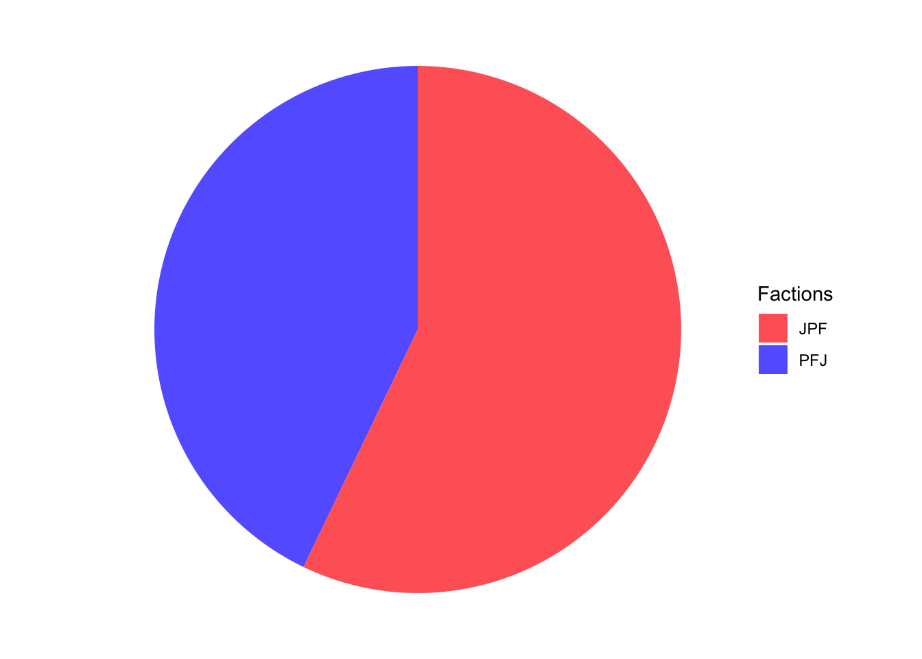
We can say that this pie chart succeeds in presenting the relative size of each faction, and to convey that these factions sum up to make the total population. Note that we are loosing information about actual number of members of each faction.
Let’s see what happens if the fractionalism among independentists increases:
table2 %>%
  kbl() %>%
kable_styling(bootstrap_options = c("striped"), full_width = FALSE)| faction | accro | men | women |
|---|---|---|---|
| People’s Front of Judea | PFJ | 40 | 45 |
| Judean People’s Front | JPF | 50 | 42 |
| Coalition for a Roman Free Judea | CRFJ | 10 | 8 |
| Social Democratic Party of Judea | SDPF | 6 | 6 |
| Judean Popular People’s Front | JPPF | 5 | 0 |
| Judean People’s Front (Maoist) | JPF-M | 15 | 12 |
| Judean Anarchist Federation | JAF | 2 | 11 |
| Front for the People’s Judea | FPJ | 8 | 6 |
| Greater Alliance for a Federated Canaa | GAFC | 7 | 5 |
To make a pie chart with total members of each faction I use mutate to create a variable summing numbers of men and women. I use fct_reorder to reorder the levels of accro by total number of members of each category, so that factions are ordered by size in the pie chart. To make the color of each faction distinctive, I am using a divergent palette of the Brewer scale. Those divergent palettes have nine categories at most, so I am pushing their possibilities to the limit here.
table2 %>%
  mutate(all = men + women) %>%
  mutate(accro = fct_reorder(accro, all, .desc = TRUE)) %>%
  ggplot(aes(x="", y = all, fill = accro)) +
  geom_bar(stat="identity", width=1) +
  coord_polar("y", start=0, direction=-1) +
  theme_void() +
  scale_fill_brewer(name = "Factions", palette = "Set1")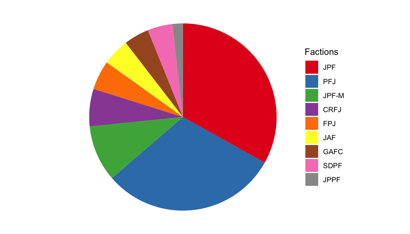
With nine categories instead of two, the pie chart is harder to read. The information about factions is presented in the legend, and the reader has to travel from legend to chart to see the weight of each faction.
This gets worse when we make a pie chart by gender using fqcet_grid. I have used across within mutate to calculate the fraction of members of each faction among men and women.
table2 %>%
  mutate(across(men:women, ~.x/sum(.x))) %>%
  mutate(accro = fct_reorder(accro, men, .desc = TRUE)) %>%
  pivot_longer(-c(faction, accro)) %>%
  ggplot(aes(x="", y = value, fill = accro)) +
  geom_bar(stat="identity", width=1) +
  coord_polar("y", start=0, direction = -1) +
  theme_void() +
  scale_fill_brewer(name = "Factions", palette = "Set1") +
  facet_grid(. ~ name)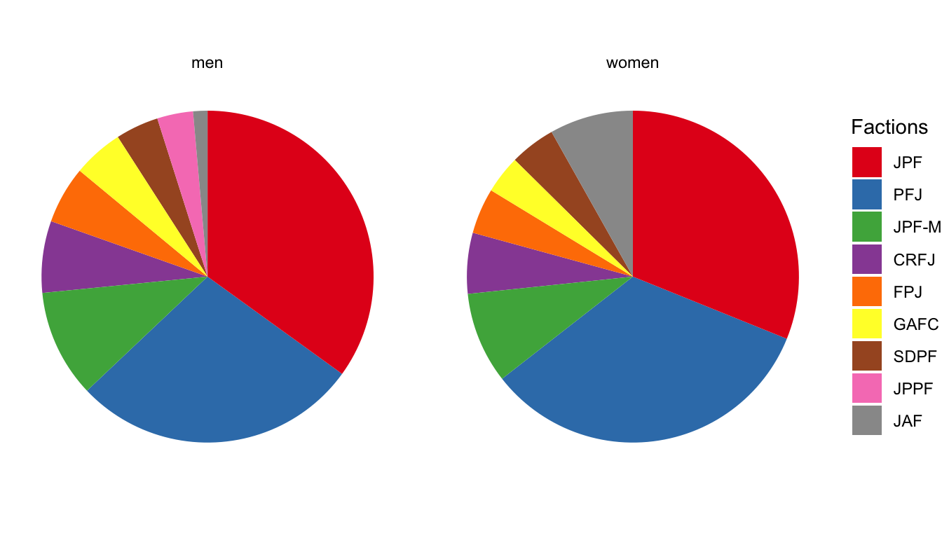
If the reader looks attentively to the pie charts, she or he can observe that the JPFF faction (in pink) is not present among women. But I think that this is far from intuitive.
Bar charts
An alternative to pie charts are bar charts. In ggplot these charts are built with geom_bar with stat = "identity". Here is a bar chart of the total members of each faction. I have used again fct_reorder to present factions with more members first.
table2 %>%
  mutate(all = men + women) %>%
  mutate(accro = fct_reorder(accro, all, .desc = FALSE)) %>%
  ggplot(aes(x= accro, y = all)) +
  geom_bar(stat = "identity", fill = "#B22222") +
  coord_flip() +
  labs(title = "Faction members", x = "faction", y = "members") +
  theme_bw()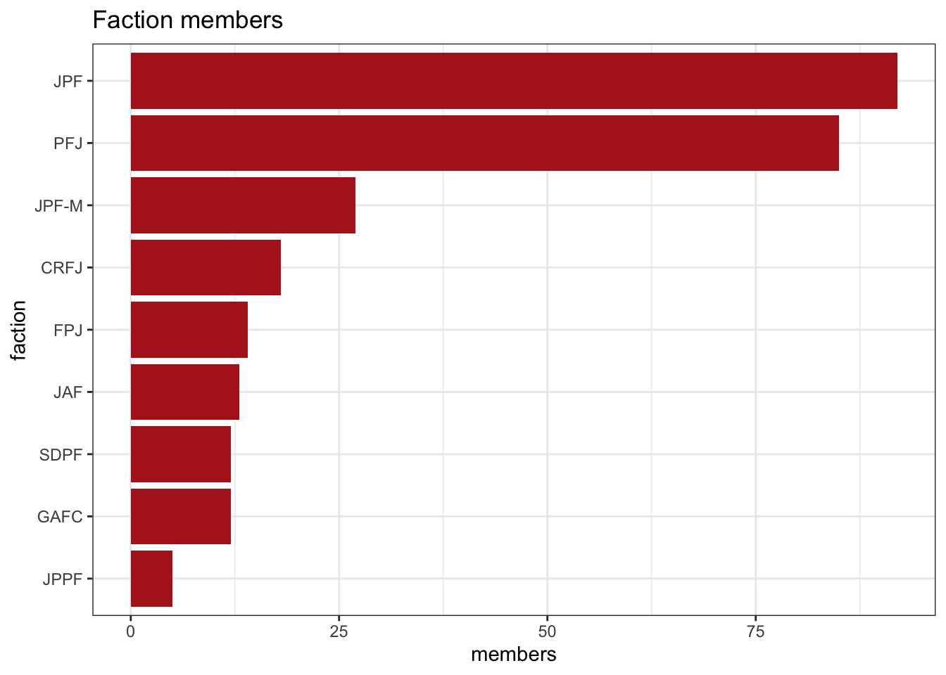
The bar chart does not convey that the sum of all members equals the total population, but each datum is linked with its label and we have information of variable values.
We can add information about men and women with a stacked bar chart. Here I use the all variable only to order bars, and fct_relevel to reverse the order of gender levels manually.
table2 %>%
  mutate(all = men + women) %>%
  mutate(accro = fct_reorder(accro, all, .desc = FALSE)) %>%
  select(-all) %>%
  pivot_longer(-c(faction, accro)) %>%
  mutate(name = fct_relevel(name, "women", "men")) %>%
  ggplot(aes(x = accro, y = value, fill = name)) +
  geom_bar(stat = "identity", position = "stack") +
  coord_flip() +
  labs(title = "Faction members by gender", x = "faction", y = "members") +
  theme_bw() +
  scale_fill_manual(name = "gender", values = c("#DC143C", "#6495ED"))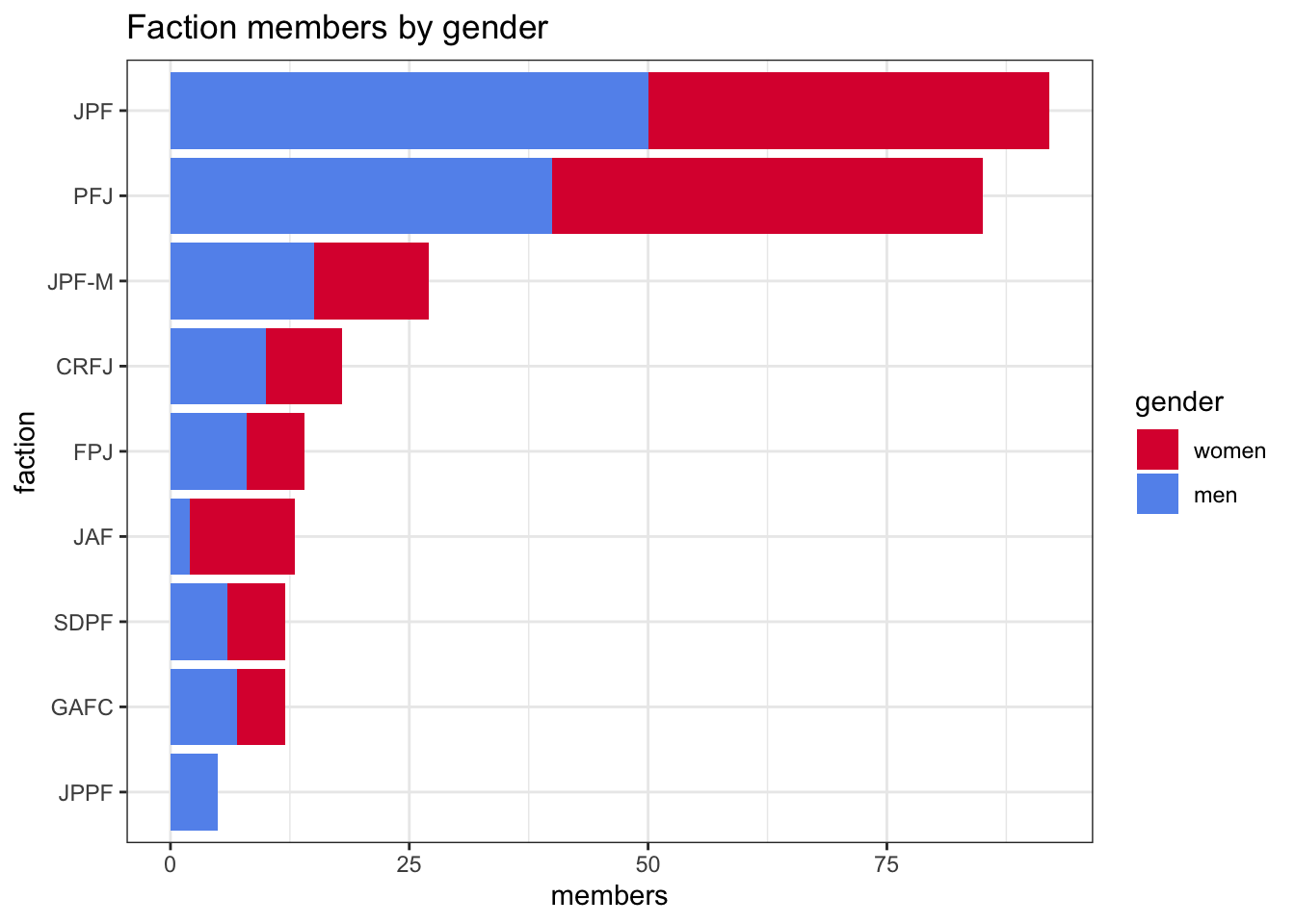
In that chart, we learn that there are no women in the JPFF faction, while the JAF faction has a large proportion of women.
We can even present faction names in the plot adding them with scale_x_discrete, and rotating them with axis.text.x. Be sure to place the theme instruction after theme_bw.
table2 %>%
  mutate(accro = fct_reorder(accro, men, .desc = TRUE)) %>%
  pivot_longer(-c(faction, accro)) %>%
  mutate(name = fct_relevel(name, "women", "men")) %>%
  ggplot(aes(x = accro, y = value, fill = name)) +
  geom_bar(stat = "identity", position = "stack") +
  labs(title = "Faction members by gender", x = "faction", y = "members") +
  theme_bw() +
  scale_fill_manual(name = "gender", values = c("#DC143C", "#6495ED")) +
  scale_x_discrete(labels = table2$faction) +
  theme(axis.text.x=element_text(angle = 90, hjust = 1, size = 10))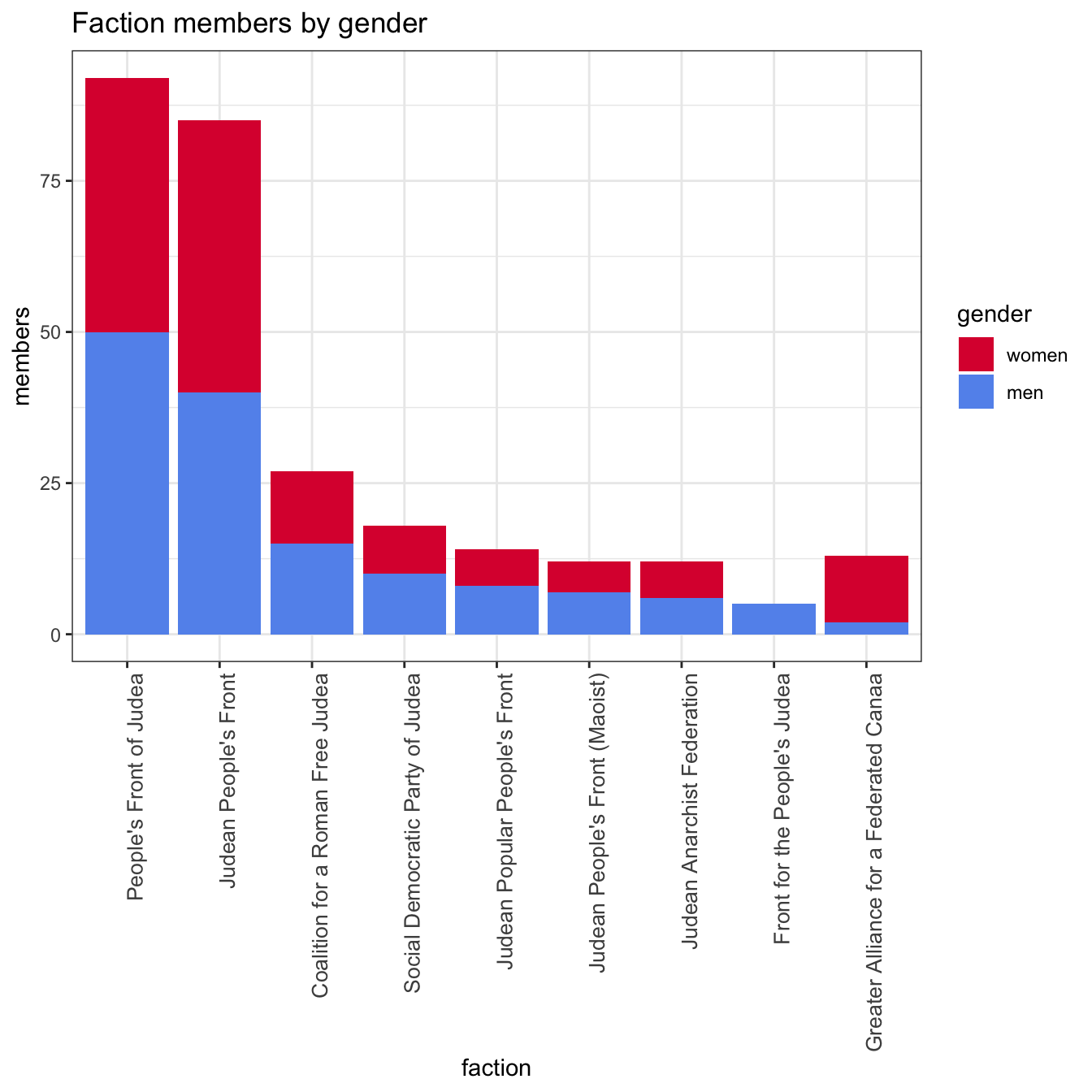
We can present the proportion of men and women participating in each faction in a single bar chart. In this case, it is more convenient to use dodged bars, as the proportion of each gender and faction is not equal to proportion of all members. I have used scales::percent in scale_y_continuous to present percentages in the y axis. Chart coordinates are reversed with coord_flip, so y axis is horizontal here.
table2 %>%
  mutate(across(men:women, ~.x/sum(.x))) %>%
  mutate(accro = fct_reorder(accro, men, .desc = FALSE)) %>%
  pivot_longer(-c(faction, accro)) %>%
  mutate(name = fct_relevel(name, "women", "men")) %>%
  ggplot(aes(x = accro, y = value, fill = name)) +
  geom_bar(stat = "identity", position = "dodge") +
  coord_flip() +
  labs(title = "Proportion of men and women in each faction", x = "faction", y = "% of members") +
  theme_bw() +
  scale_fill_manual(name = "gender", values = c("#DC143C", "#6495ED")) +
  scale_y_continuous(labels = scales::percent)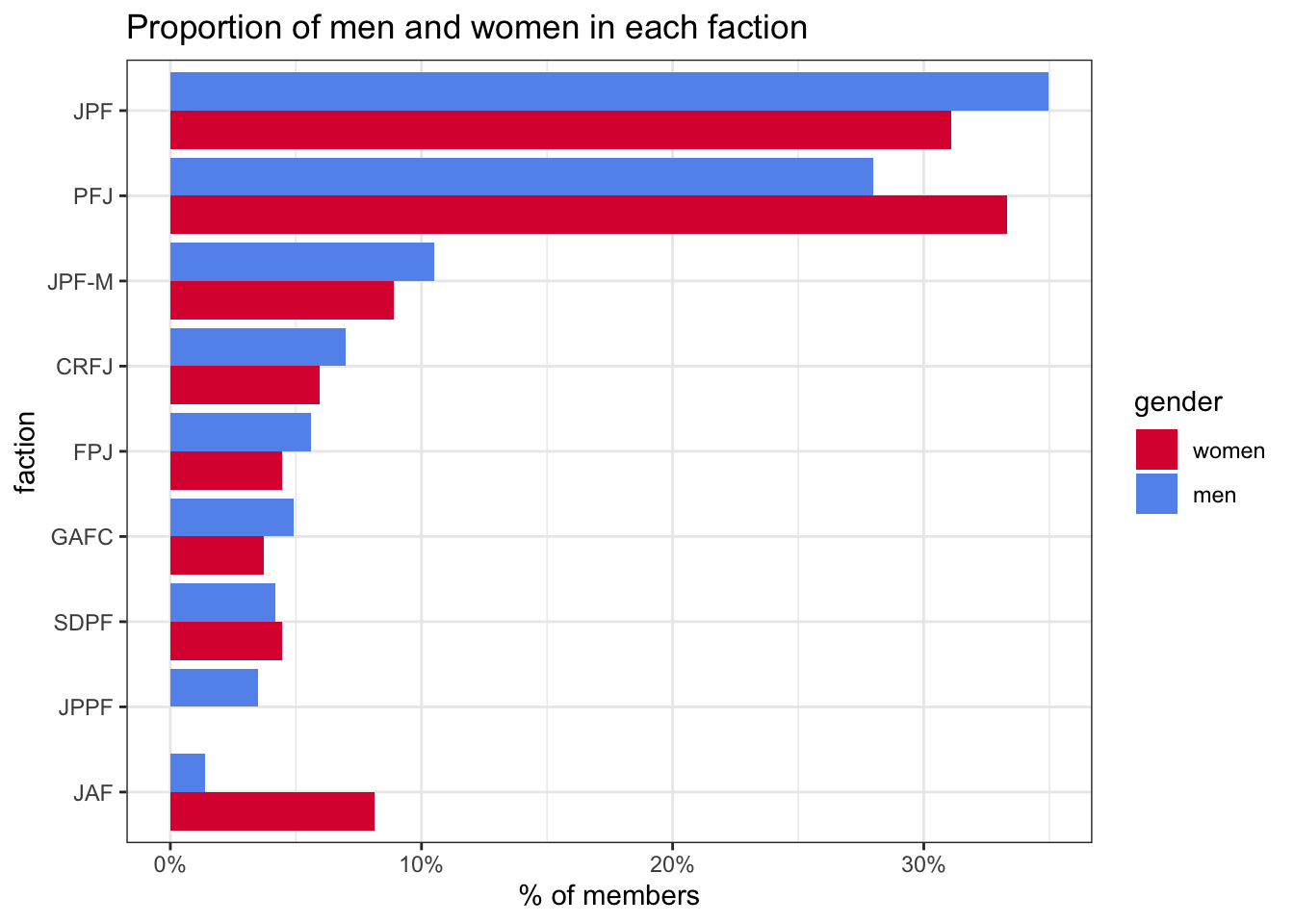
Here we learn that the JPF faction is the preferred among men, while PFJ is the preferred among women.
Pie or bar charts?
Examinimg the possibilities of pie charts and bars, most people tend to prefer bar charts, like in this post. We can use pie charts when the part-to-whole comparison is of interest, and the number of categories is relatively small. Bar charts are preferable to represent more complex relationships of data, involving more than one category, or when the number of categories is high.
References
- The R Graph Gallery (n.d). R Color Brewer’s palettes https://www.r-graph-gallery.com/38-rcolorbrewers-palettes.html
- Reddit (n.d.). What led to the split between the People’s Front of Judea and the Judean People’s Front in the first century? https://www.reddit.com/r/AskHistorians/comments/30yfs7/what_led_to_the_split_between_the_peoples_front/
Built with R 4.0.3 and tidyverse 1.3.0