Pareto Front in Multicriteria Optimization

Jose M Sallan 2024-06-13 8 min read

In this post, I will introduce the concept of Pareto optimal solutions and Pareto front in the context of multicriteria optimization. I will present the concept with the mtcars dataset, and code a function detecting Pareto optimal solutions as an example of application of the data.table package. Finally, I will present the rPref package which allows detecting Pareto optimal solutions effectively.

library(data.table)
library(rPref)
library(ggplot2)

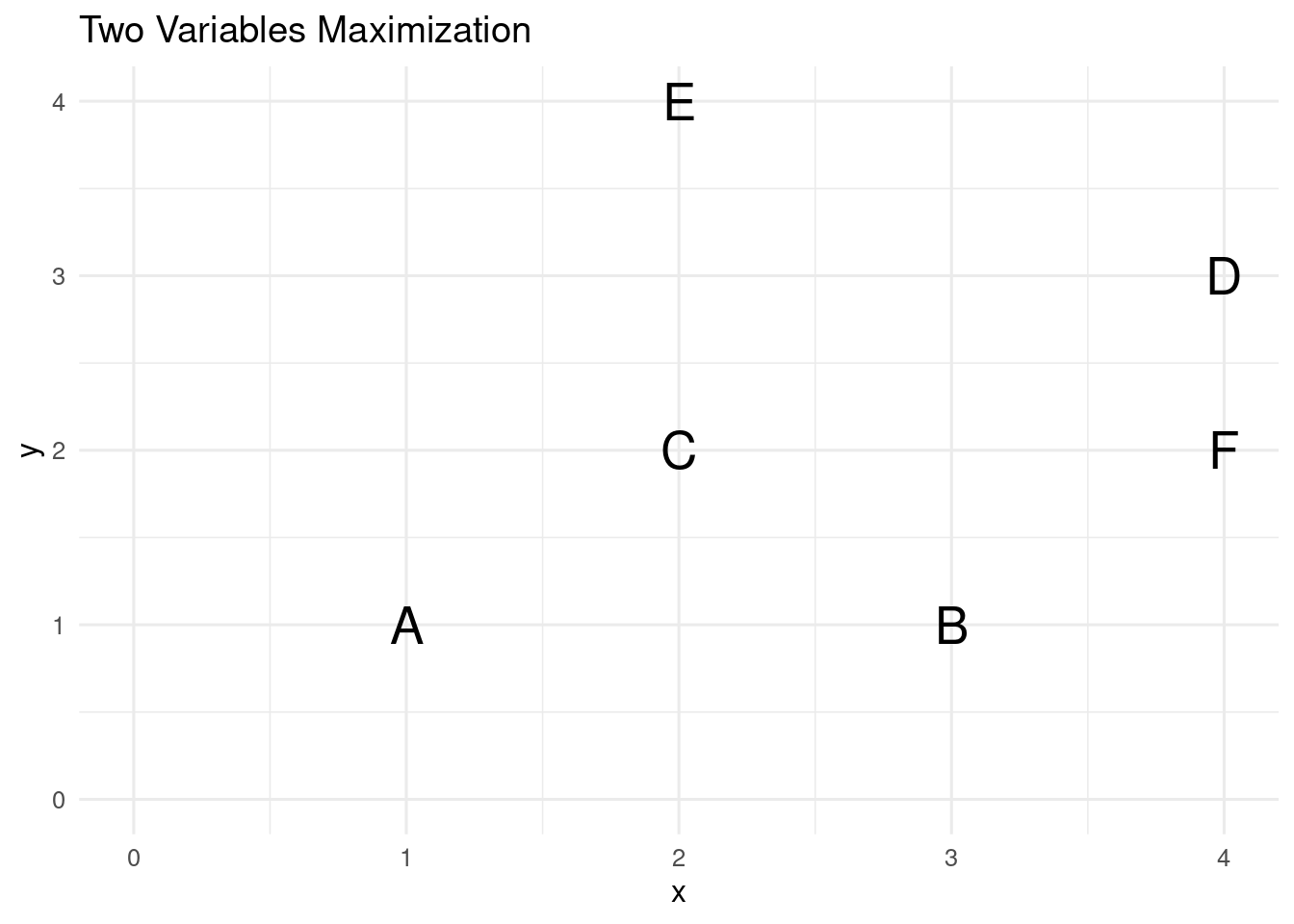
Let’s start with a toy example, in which we have the values of two variables for a set of six elements.

small_example <- data.table(name = LETTERS[1:6],
                            x = c(1, 3, 2, 4, 2, 4),
                            y = c(1, 1, 2, 3, 4, 2))

Let’s suppose that we want variables with high values of x and high values of y. This is a case of multicriteria optimization, as we want to maximize two variables simultaneously.

small_example |>
  ggplot(aes(x, y, label = name)) +
  xlim(0, 4) +
  ylim(0, 4) +
  geom_text(size = 7) +
  theme_minimal(base_size = 12) +
  labs(title = "Two Variables Maximization")

Examining the plot of values of x versus y lead us to discard some of the solutions. One of these is C, as solution D has better values of x and y. We can say that solution D dominates solution C. More precisely, we say that a solution \(s_i\) dominates a solution \(s_j\) when:

\(s_i\) has equal or better values than \(s_j\) in all variables.
\(s_i\) is strictly better than \(s_j\) in at least one variable.

With this criterion, we observe that D also dominates F: both solutions have the same value of x, but D has a better value of y.

If we check for dominance relationships for all pairs of solutions, we will end up knowking that solutions D and E are not dominated by any other solution. These solutions are Pareto efficient: when choosing betweeen them, we cannot increase the value of one decision variable without reducing the value of the other variable, so choosing between them is a trade-off. The set of Pareto efficient solutions is the Pareto front.

This definition of Pareto front can be extended to more than two variables, and each variable can be either maximized or minimized.

Let’s define a pf() function to detect Pareto efficient solutions for two variables using data.table.

pf <- function(tab, v, type = "high"){
  
  # copying the input table to not modify it
  tab0 <- copy(tab)
  
  # selecting columns
  tab1 <- tab0[ , ..v]
  
  # defining id
  tab1[, name := 1:nrow(tab1)]
  
  # defining all Pareto comparison
  pareto <- CJ(tab1[, name], tab1[, name])[V1 != V2]
  
  # adding values of first variable
  pareto <- merge(pareto, tab1,
                  by.x = "V1", by.y = "name")
  
  # adding values of second variable
  pareto <- merge(pareto, tab1,
                  by.x = "V2", by.y = "name")
  
  # matrices of values of v2 and v1
  values_v2 <- as.matrix(pareto[, 5:6])
  values_v1 <- as.matrix(pareto[, 3:4])

  # checking if solution v2 dominates solution v1
  if(type == "high"){
    pareto[, domin := 
             sapply(1:nrow(pareto), function(i) all(values_v1[i, ] <= values_v2[i, ]) &
                      any(values_v1[i, ] < values_v2[i, ]))]
  }else{
    pareto[, domin := 
             sapply(1:nrow(pareto), function(i) all(values_v1[i, ] >= values_v2[i, ]) &
                               any(values_v1[i, ] > values_v2[i, ]))]
  }
  
  # column with dominated solutions
  pareto[, domin_sol := ifelse(domin, V1, 0)]

  # extracting dominated solutions
  domin <- pareto[domin_sol != 0, domin_sol] |>
    unique()
  
  pf <- tab0[!tab1[, name] %in% domin]
  
  return(pf)
}

This function works as follows:

From the input table tab, we retain the columns specified in vector v.
We define the pareto table, with all combinations of pairs of different observations.
For each row of pareto, we examine if solution v2 dominates solution v1. If this is true, we add the value of v1 in the column domin_sol.
We obtain the vector domin of unique dominated solutions.
We return the Pareto frontier as the set of observations not contained in domin.

If we apply this function to our example, we obtain:

pf(tab = small_example, v = c("x", "y"), type = "high")

##      name     x     y
##    <char> <num> <num>
## 1:      D     4     3
## 2:      E     2     4

Miles per Gallon versus Horsepower

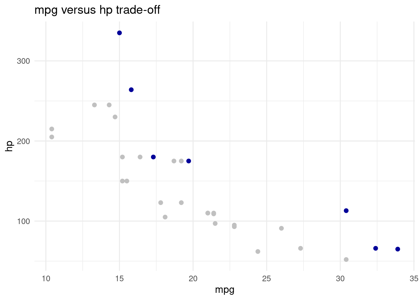
Let’s suppose that we want to choose the values of mtcars which maximize miles per gallon and gross horsepower. Let’s transform mtcars so that we can use our function:

mtcars0 <- data.table(mtcars)
mtcars0[, c("name", "l100km") := .(row.names(mtcars), 235.214583/mpg)]

Then we obtain:

mtcars_mpg_hp <- pf(mtcars0, v = c("mpg", "hp"), type = "high")
mtcars_mpg_hp[ ,.(name, mpg, hp)]

##              name   mpg    hp
##            <char> <num> <num>
## 1:     Merc 450SL  17.3   180
## 2:       Fiat 128  32.4    66
## 3: Toyota Corolla  33.9    65
## 4:   Lotus Europa  30.4   113
## 5: Ford Pantera L  15.8   264
## 6:   Ferrari Dino  19.7   175
## 7:  Maserati Bora  15.0   335

Not suprisingly, we obtain a combination of sports cars like Ferrari Dino and small cars like Fiat 128. Our choice between these cars will depend on the value we put to fuel consumption and horsepower.

Let’s see how the Pareto frontier looks like.

mtcars0[, pf1 := ifelse(name %in% mtcars_mpg_hp[, name], "yes", "no")]
ggplot(mtcars0, aes(mpg, hp, color = pf1)) +
  geom_point(size = 2) +
  scale_color_manual(values = c("#C0C0C0", "#000099")) +
  theme_minimal(base_size = 12) +
  theme(legend.position = "none") +
  labs(title = "mpg versus hp trade-off")

Liters per 100 Kilometer versus 1/4 Mile Time

Let’s find the Pareto front of:

Minimizing fuel consumption in liters per 100 kilometer.
Minimize the time to run 1/4 mile, a measure of acceleration.

mtcars_l100_qsec <- pf(mtcars0, v = c("l100km", "qsec"), type = "low")
mtcars_l100_qsec[ ,.(name, l100km, qsec)]

##              name    l100km  qsec
##            <char>     <num> <num>
## 1:      Mazda RX4 11.200694 16.46
## 2:       Fiat 128  7.259709 19.47
## 3: Toyota Corolla  6.938483 19.90
## 4:  Porsche 914-2  9.046715 16.70
## 5:   Lotus Europa  7.737322 16.90
## 6: Ford Pantera L 14.886999 14.50
## 7:   Ferrari Dino 11.939827 15.50

We observe again a combination of sports cars and small cars, representing the tradeoff between fuel consumption and engine performance.

This Pareto front looks as follows:

mtcars0[, pf2 := ifelse(name %in% mtcars_l100_qsec[, name], "yes", "no")]
ggplot(mtcars0, aes(l100km, qsec, color = pf2)) +
  geom_point(size = 2) +
  scale_color_manual(values = c("#C0C0C0", "#990000")) +
  theme_minimal(base_size = 12) +
  theme(legend.position = "none") +
  labs(title = "l100km versus qsec trade-off")

The rPref Package

The rPref package allows fast computation of Pareto fronts for any combination of variables. These are obtained with the psel() function. Let’s use it to obtain the values of mpg versus hp in mtcars:

psel(mtcars0, high(mpg)*high(hp))[, .(name, mpg, hp)]

##              name   mpg    hp
##            <char> <num> <num>
## 1:     Merc 450SL  17.3   180
## 2:       Fiat 128  32.4    66
## 3: Toyota Corolla  33.9    65
## 4:   Lotus Europa  30.4   113
## 5: Ford Pantera L  15.8   264
## 6:   Ferrari Dino  19.7   175
## 7:  Maserati Bora  15.0   335

And the values of l100km versus qsec:

psel(mtcars0, low(l100km)*low(qsec))[, .(name, l100km, qsec)]

##              name    l100km  qsec
##            <char>     <num> <num>
## 1:      Mazda RX4 11.200694 16.46
## 2:       Fiat 128  7.259709 19.47
## 3: Toyota Corolla  6.938483 19.90
## 4:  Porsche 914-2  9.046715 16.70
## 5:   Lotus Europa  7.737322 16.90
## 6: Ford Pantera L 14.886999 14.50
## 7:   Ferrari Dino 11.939827 15.50

We can explore more sophisticated criteria like:

psel(mtcars0, low(l100km)*low(qsec)*high(hp))[, .(name, l100km, qsec, hp)]

##               name    l100km  qsec    hp
##             <char>     <num> <num> <num>
##  1:      Mazda RX4 11.200694 16.46   110
##  2:     Merc 450SE 14.342353 17.40   180
##  3:     Merc 450SL 13.596219 17.60   180
##  4:       Fiat 128  7.259709 19.47    66
##  5: Toyota Corolla  6.938483 19.90    65
##  6:  Porsche 914-2  9.046715 16.70    91
##  7:   Lotus Europa  7.737322 16.90   113
##  8: Ford Pantera L 14.886999 14.50   264
##  9:   Ferrari Dino 11.939827 15.50   175
## 10:  Maserati Bora 15.680972 14.60   335

Note that when we include more criteria the number of Pareto solutions tends to increase, as it is harder that a solution could be dominated by other in all criteria.

Pareto Front and Multicriteria Optimization

When we optimize a function with a single criterion, we obtain a single solution (or a set of solution with the same optimal value of the objective function). When we optimize with two or more criteria, our result is a set of non-dominated solutions called the Pareto front. The solutions of this set are Pareto optimal: when going from one solution to other we cannot improve one criterion without deteriorating others.

We usually see Pareto fronts with two variables, as they are easy to plot to present Pareto optimality, but we can optimize more than two variables. The more variables to optimize, the harder that a solution will be dominated by other in all criteria will be, so that the Pareto front will tend to be larger.

References

rPref package (R Journal) https://journal.r-project.org/archive/2016-2/roocks.pdf
rPref package (website): https://www.p-roocks.de/rpref/

Session Info

## R version 4.4.0 (2024-04-24)
## Platform: x86_64-pc-linux-gnu
## Running under: Linux Mint 21.1
## 
## Matrix products: default
## BLAS:   /usr/lib/x86_64-linux-gnu/blas/libblas.so.3.10.0 
## LAPACK: /usr/lib/x86_64-linux-gnu/lapack/liblapack.so.3.10.0
## 
## locale:
##  [1] LC_CTYPE=es_ES.UTF-8       LC_NUMERIC=C              
##  [3] LC_TIME=es_ES.UTF-8        LC_COLLATE=es_ES.UTF-8    
##  [5] LC_MONETARY=es_ES.UTF-8    LC_MESSAGES=es_ES.UTF-8   
##  [7] LC_PAPER=es_ES.UTF-8       LC_NAME=C                 
##  [9] LC_ADDRESS=C               LC_TELEPHONE=C            
## [11] LC_MEASUREMENT=es_ES.UTF-8 LC_IDENTIFICATION=C       
## 
## time zone: Europe/Madrid
## tzcode source: system (glibc)
## 
## attached base packages:
## [1] stats     graphics  grDevices utils     datasets  methods   base     
## 
## other attached packages:
## [1] ggplot2_3.5.1     rPref_1.4.0       data.table_1.15.4
## 
## loaded via a namespace (and not attached):
##  [1] gtable_0.3.5       jsonlite_1.8.8     highr_0.10         dplyr_1.1.4       
##  [5] compiler_4.4.0     tidyselect_1.2.1   Rcpp_1.0.12        jquerylib_0.1.4   
##  [9] scales_1.3.0       yaml_2.3.8         fastmap_1.1.1      R6_2.5.1          
## [13] labeling_0.4.3     generics_0.1.3     igraph_2.0.3       knitr_1.46        
## [17] tibble_3.2.1       bookdown_0.39      munsell_0.5.1      bslib_0.7.0       
## [21] pillar_1.9.0       rlang_1.1.3        utf8_1.2.4         cachem_1.0.8      
## [25] xfun_0.43          sass_0.4.9         lazyeval_0.2.2     RcppParallel_5.1.7
## [29] cli_3.6.2          withr_3.0.0        magrittr_2.0.3     digest_0.6.35     
## [33] grid_4.4.0         rstudioapi_0.16.0  lifecycle_1.0.4    vctrs_0.6.5       
## [37] evaluate_0.23      glue_1.7.0         farver_2.1.1       blogdown_1.19     
## [41] colorspace_2.1-0   fansi_1.0.6        rmarkdown_2.26     tools_4.4.0       
## [45] pkgconfig_2.0.3    htmltools_0.5.8.1

The Jose M Sallan static website