Acquiring the ulysses16 instance

The ulysses16 instance consists of 16 locations of The Oddyssey, presented in Grötschel & Padberg (2001). Our task is help Ulysses to travel the minimal possible distance solving the TSP for these 16 locations.

To start with, we need to retrieve the data from TSP-LIB (Reinelt, 1991). The code below proceeds as follows:

• I am retrieving the dataset from the Internet using readLines, and retaninng the part of the text containing the coordinates.
• I use strpslit to obtain the elements between spaces for each line of the coordinates. Latitude and longitude are the third and fourth element of each line, respectively. I am storing them in coord_lat and coord_lon, respectively.
• In Reinelt (1991) we learn that coordinates are presented as DD.MM, where DD are degrees and MM minutes. So we need to obtain decimal degrees with the min_to_dec function.
• I store the transformed values of latitude and longitude in a tibble, a modified data frame used in the Tidyverse.

data <- readLines("http://elib.zib.de/pub/mp-testdata/tsp/tsplib/tsp/ulysses16.tsp")
bof <- which(data == "NODE_COORD_SECTION") + 1
eof <- which(data==" EOF") - 1

data <- data[bof:eof]
data_split <- strsplit(data, " ")

coord_lat <- sapply(data_split, function(x) as.numeric(x[3]))
coord_lon <- sapply(data_split, function(x) as.numeric(x[4]))

min_to_dec <- function(x){
  
  deg <- trunc(x)
  min <- (x - trunc(x)) * 100
  
  dec <- deg + min/60
  
}

coord_lat <- min_to_dec(coord_lat)
coord_lon <- min_to_dec(coord_lon)

n <- length(coord_lat)

coords <- tibble(id =1:n, lat = coord_lat, lon = coord_lon)

To calculate distances between two points on the surface of the Earth we can use the distGeo function of the geosphere package. It is important to notice that each point has to be entered in longitude / latitude format. If we take this into account, the distances obtained are similar to the results of the formula in Reinelt (1991).

distances <- matrix(0, nrow = n, ncol = n)

for(i in 1:n)
  for(j in 1:n){
    x <- c(coords[i,]$lon, coords[i,]$lat)
    y <- c(coords[j,]$lon, coords[j,]$lat)
    distances[i, j] <- round(distGeo(x, y)/1000)
  }

The Miller-Tucker-Zemlin formulation of the travelling salesman problem

Now is time to solve the travelling salesman problem (TSP). Given a matrix of distances between nodes, the solution of the TSP is the shortest cycle that visits each city exactly once.

A classical formulation of this problem is the one presented in Miller, Tucker and Zemlin (1960), often called the MZT formulation. It has two sets of variables:

• Variables \(x_{ij}\), for all ordered pairs \(i = 1, \dots, n\), \(j = 1, \dots, n\) and \(i \neq j\). \(n\) is the number of nodes. These variables are equal to one if the directed arc \(\left( i, j \right)\) belongs to the solution, and zero otherwise.
• Variables \(u_i\) with \(i=2, \dots, n\), used for the subtour elimination constraints.

The objective function is defined as:

\[ \text{MIN } z = \sum_{i=1}^n \sum_{j=1}^n d_{ij}x_{ij}\]

In the solution, exactly one edge must depart from each node:

\[ \sum_{j=1}^n x_{ij} = 1, \ \ i = 1, \dots, n\]

and one edge must arrive to each node:

\[ \sum_{i=1}^n x_{ij} = 1, \ \ j = 1, \dots, n\]

We use variables \(u_i\) to eliminate subtours:

\[ u_j - u_i + nx_{ij} \leq n-1,\ \ i = 2, \dots ,n,\ \ j = 2, \dots, n \]

These variables are defined for all nodes except \(i=1\), which is chosen arbitrarily. For pairs of edges where \(x_{ij} = 1\), the constraint works as \(u_j - u_i \leq -1\). For the remaining \(x_{ij} = 0\) the constraint works as \(u_j - u_i \leq n-1\). The result is that \(u_i\) increases as node \(i\) separates from node 1 in the solution, so that the tour can only close on node 1. As the value of the first \(u_i\) can be arbitrary, I have bounded \(u_i\) variables to take values between 1 and \(n-1\).

I am using the ompr package to define a mixed integer linear programming model. We can add_variable, set_objective and add_constraint straight from the R environment. The parameters of the model are the number of nodes n and the distances matrix.

model <- MIPModel() %>%
  
  # we create a variable that is 1 iff we travel from node i to j
  add_variable(x[i, j], i = 1:n, j = 1:n, i != j, type = "binary") %>%
  
  # helper variable for the MTZ sub-tour constraints
  add_variable(u[i], i = 2:n, lb = 1, ub = n-1) %>%
  
  # minimize travel distance and latest arrival
  set_objective(sum_over(distances[i, j] * x[i, j], i = 1:n, j = 1:n, i != j), "min") %>%

  # leave each city exactly once
  add_constraint(sum_over(x[i, j], j = 1:n, i != j) == 1, i = 1:n) %>%
  
  # arrive at each city exactly once
  add_constraint(sum_over(x[i, j], i = 1:n, i != j) == 1, j = 1:n) %>%
  
  # ensure no subtours (arc constraints)
  add_constraint(u[i] - u[j] + n*x[i, j] <= n-1, i = 2:n, j = 2:n, i != j)

Solving the ulysses16 instance

I am using the ompr.roi and the ROI.plugin.glpk packages to solve the model using the GLPK library. The solution is stored in the result object.

result <- solve_model(model, with_ROI(solver = "glpk"))
result

## Status: success
## Objective value: 6855

We can extract the variables of the solution using get_solution. Here I am extracting the values of \(x_{ij} = 1\):

solution <- get_solution(result, x[i, j]) %>%
  filter(value > 0)
solution

##    variable  i  j value
## 1         x  8  1     1
## 2         x  3  2     1
## 3         x 16  3     1
## 4         x  2  4     1
## 5         x 15  5     1
## 6         x  7  6     1
## 7         x 12  7     1
## 8         x  4  8     1
## 9         x 11  9     1
## 10        x  9 10     1
## 11        x  5 11     1
## 12        x 13 12     1
## 13        x 14 13     1
## 14        x  1 14     1
## 15        x  6 15     1
## 16        x 10 16     1

If we extract the values of \(u_i\) we observe that they increase as we depart from node 1:

get_solution(result, u[i]) %>%
  arrange(value)

##    variable  i value
## 1         u 14     1
## 2         u 13     2
## 3         u 12     3
## 4         u  7     4
## 5         u  6     5
## 6         u 15     6
## 7         u  5     7
## 8         u 11     8
## 9         u  9     9
## 10        u 10    10
## 11        u 16    11
## 12        u  3    12
## 13        u  2    13
## 14        u  4    14
## 15        u  8    15

The objective function and the solution are the same as the reported in TSP-LIB: http://elib.zib.de/pub/mp-testdata/tsp/tsplib/tsp/ulysses16.opt.tour

Plotting the solution

Let’s add latitude and longitude to each point of the solution to plot the segments on a map:

solution <- left_join(solution, coords, by = c("i" = "id")) %>%
  rename(lati = lat, loni = lon)

solution <- left_join(solution, coords, by = c("j" = "id")) %>%
  rename(latj = lat, lonj = lon)

This code allows presenting the geographical positions of the optimal tour:

• I am setting the range of the world map to present with coord_sf. These values are usually obtained through trial and error.
• The nodes are plotted with the information of the coords table.
• The segments are plotted with the information of the solution table.

ggplot(WorldMap1_10) +
  geom_sf(fill = "#F5DEB3") +
  coord_sf(xlim = c(-6, 28), ylim = c(30, 45)) +
  geom_point(data = coords, aes(lon, lat)) +
  geom_segment(data = solution, aes(x = loni, y = lati, xend = lonj, yend = latj)) +
  theme_void() +
  theme(plot.background = element_rect(fill = '#CCFFFF'))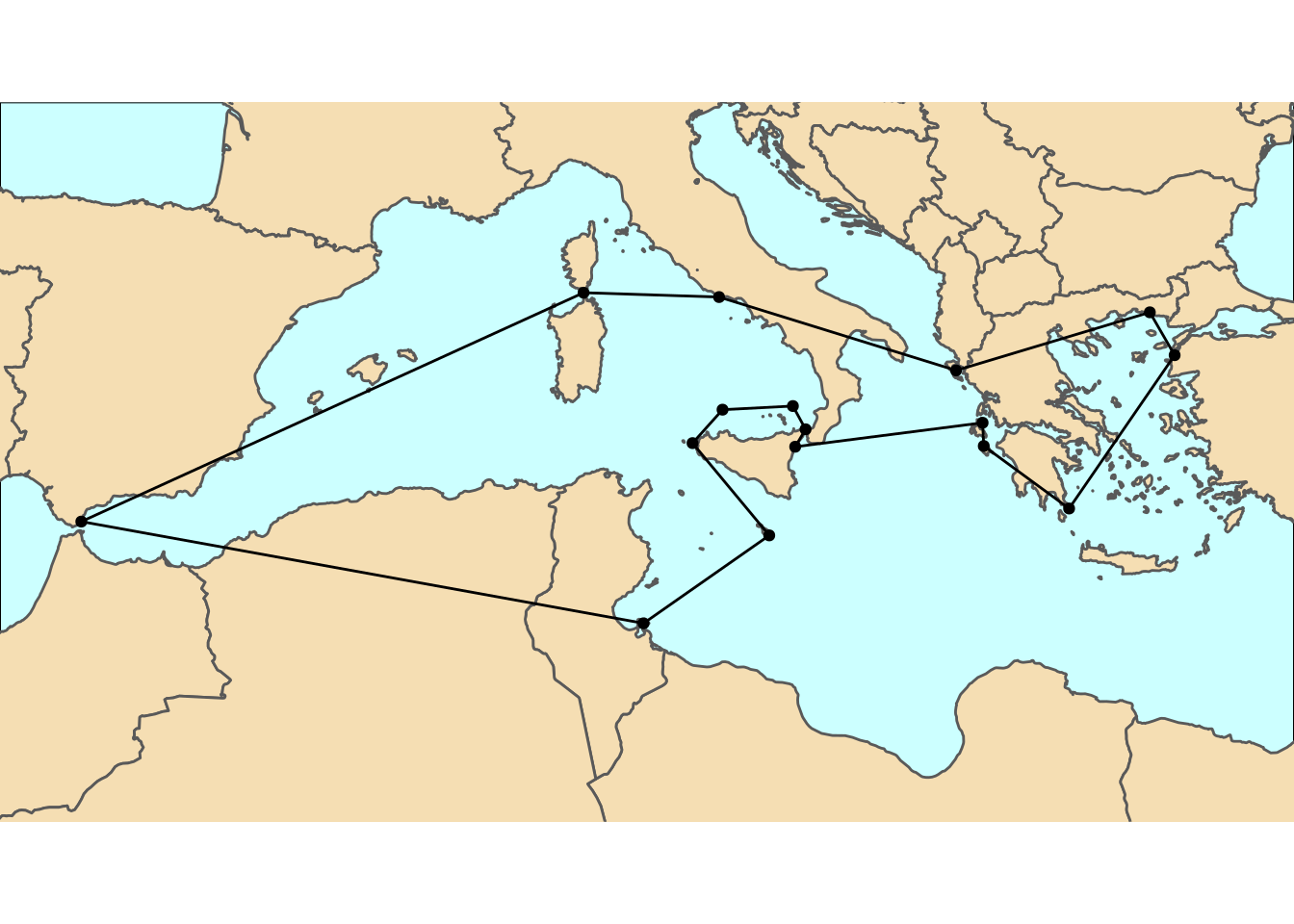

Acknowledgements

Thanks again to Mari Albareda for proofreading the text and correcting the mistakes of the MZT formulation of an earlier version of this post. All remaining errors are my own.

References

• AIMS (2022). The Miller-Tucker-Zeimlin formulation. https://how-to.aimms.com/Articles/332/332-Miller-Tucker-Zemlin-formulation.html
• Reinelt, G. (1991). TSPLIB—A Traveling Salesman Problem Library. ORSA Journal on Computing, 3(4):376-384. https://doi.org/10.1287/ijoc.3.4.376
• Grötschel, M., & Padberg, M. (2001). The Optimized Odyssey. AIROnews VI, 2, 1-7.
• Miller, C. E., Tucker, A. W., & Zemlin, R. A. (1960). Integer programming formulation of traveling salesman problems. Journal of the ACM (JACM), 7(4), 326-329. https://doi.org/10.1145/321043.321046

Session info

## R version 4.1.2 (2021-11-01)
## Platform: x86_64-pc-linux-gnu (64-bit)
## Running under: Debian GNU/Linux 10 (buster)
## 
## Matrix products: default
## BLAS:   /usr/lib/x86_64-linux-gnu/blas/libblas.so.3.8.0
## LAPACK: /usr/lib/x86_64-linux-gnu/lapack/liblapack.so.3.8.0
## 
## locale:
##  [1] LC_CTYPE=es_ES.UTF-8       LC_NUMERIC=C              
##  [3] LC_TIME=es_ES.UTF-8        LC_COLLATE=es_ES.UTF-8    
##  [5] LC_MONETARY=es_ES.UTF-8    LC_MESSAGES=es_ES.UTF-8   
##  [7] LC_PAPER=es_ES.UTF-8       LC_NAME=C                 
##  [9] LC_ADDRESS=C               LC_TELEPHONE=C            
## [11] LC_MEASUREMENT=es_ES.UTF-8 LC_IDENTIFICATION=C       
## 
## attached base packages:
## [1] stats     graphics  grDevices utils     datasets  methods   base     
## 
## other attached packages:
## [1] BAdatasetsSpatial_0.1.0 sf_1.0-2                geosphere_1.5-14       
## [4] ROI.plugin.glpk_1.0-0   ompr.roi_1.0.0          ompr_1.0.2             
## [7] ggplot2_3.3.5           dplyr_1.0.7            
## 
## loaded via a namespace (and not attached):
##  [1] Rcpp_1.0.6          lattice_0.20-45     class_7.3-19       
##  [4] assertthat_0.2.1    digest_0.6.27       utf8_1.2.1         
##  [7] slam_0.1-49         R6_2.5.0            evaluate_0.14      
## [10] e1071_1.7-8         highr_0.9           blogdown_1.5       
## [13] pillar_1.6.4        rlang_0.4.12        lazyeval_0.2.2     
## [16] data.table_1.14.0   jquerylib_0.1.4     Matrix_1.3-4       
## [19] rmarkdown_2.9       listcomp_0.4.1      stringr_1.4.0      
## [22] munsell_0.5.0       proxy_0.4-26        ROI_1.0-0          
## [25] compiler_4.1.2      numDeriv_2016.8-1.1 xfun_0.23          
## [28] pkgconfig_2.0.3     Rglpk_0.6-4         htmltools_0.5.1.1  
## [31] tidyselect_1.1.1    tibble_3.1.5        bookdown_0.24      
## [34] fansi_0.5.0         crayon_1.4.1        withr_2.4.2        
## [37] wk_0.5.0            grid_4.1.2          jsonlite_1.7.2     
## [40] gtable_0.3.0        lifecycle_1.0.0     registry_0.5-1     
## [43] DBI_1.1.1           magrittr_2.0.1      units_0.7-2        
## [46] scales_1.1.1        KernSmooth_2.23-20  stringi_1.7.3      
## [49] farver_2.1.0        sp_1.4-5            bslib_0.2.5.1      
## [52] ellipsis_0.3.2      generics_0.1.0      vctrs_0.3.8        
## [55] s2_1.0.6            tools_4.1.2         glue_1.4.2         
## [58] purrr_0.3.4         fastmap_1.1.0       yaml_2.2.1         
## [61] colorspace_2.0-1    classInt_0.4-3      knitr_1.33         
## [64] sass_0.4.0