Linear Programming Formulation

Let’s define a formulation for this problem that avoids symmetry. Our input will be the graph \(G(N, E)\) of \(n\) nodes and \(e\) edges.

The decision variables will be of the type \(w_{ij}\), which are equal to one if node \(j\) belongs to the set of nodes with the same label with lowest index equal to \(i\). Then, in those variables \(i \leq j\).

Defined in this way, our objective function will be minimizing the sum of variables \(w_{ii}\).

The constraints will be:

• Variables \(w_{ij}\) must be lower or equal than \(w_{ii}\), so that \(w_{ij} = 0\) when \(w_{ii} = 0\).
• Each node \(j\) must have a single label.
• Pairs of nodes \((j,k)\) defining vertexs of \(E\) must have different color.

\(\begin{align} \text{MIN } & z = \sum_{i=1}^n w_{ii} \\ & w_{ij} \leq w_{ii} & i = 1, \dots, n, \ i \leq j \\ & \sum_{i=1}^j w_{ij} = 1 & j = 1, \dots, n \\ & w_{ij} + w_{ik} \leq 1 & (j, k) \in E, \ i \leq j, \ i \leq k \\ \end{align}\)

The Barcelona Districts Map

Let’s color the map of districts of Barcelona. It is delivered as a spatial object BCNDistricts, so it is a data frame with a geometry column where are stored the polygons to draw the districts. I will order this dataframe by the district numerical code c_distri.

data("BCNDistricts")

BCNDistricts <- BCNDistricts |>
  arrange(c_distri)

Let’s plot the map with the values of c_distri.

BCNDistricts |>
  ggplot() +
  geom_sf() +
  geom_text(aes(coord_x, coord_y, label = c_distri)) +
  theme_void()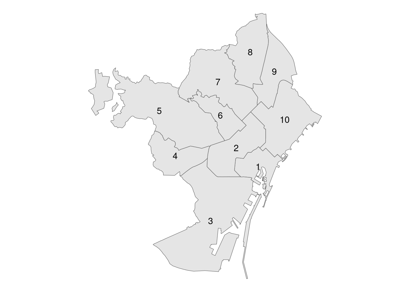

Finding the contacts among districts can be tedious. Fortunately, districts are stored as simple feature geometrical objects. We can use the sf::st_touches() function to see which objects contact each other:

int <- st_touches(BCNDistricts)
int

## Sparse geometry binary predicate list of length 10, where the predicate
## was `touches'
##  1: 2, 3, 10
##  2: 1, 3, 4, 5, 6, 7, 10
##  3: 1, 2, 4
##  4: 2, 3, 5
##  5: 2, 4, 6, 7
##  6: 2, 5, 7
##  7: 2, 5, 6, 8, 9, 10
##  8: 7, 9
##  9: 7, 8, 10
##  10: 1, 2, 7, 9

Note that the values of int are the row number of the districts, not necessarily values of c_distri. That is why I have arranged rows by this variable previously.

Iterating with purrr::map_dfr() we can obtain the list of edges:

edges_col <- map_dfr(1:length(int), ~ tibble(i = ., j = int[[.]])) |>
  filter(i < j)
edges_col

## # A tibble: 19 × 2
##        i     j
##    <int> <int>
##  1     1     2
##  2     1     3
##  3     1    10
##  4     2     3
##  5     2     4
##  6     2     5
##  7     2     6
##  8     2     7
##  9     2    10
## 10     3     4
## 11     4     5
## 12     5     6
## 13     5     7
## 14     6     7
## 15     7     8
## 16     7     9
## 17     7    10
## 18     8     9
## 19     9    10

So we have 19 edges and 10 nodes for this node coloring problem.

Solving the Problem

Let’s define the linear programming model to solve this problem, based on the formulation. We start defining the number of nodes and edges.

n <- length(unique(c(edges_col$i, edges_col$j)))
e <- nrow(edges_col)

Here is the model, built with the OMPR syntax. Note that it is using the values of edges_col to define the specific model for this case.

gc_model <- 
  MIPModel() |>
  add_variable(w[i, j], i = 1:n, j = 1:n, i<=j, type = "binary") |>
  add_constraint(w[i, j] <= w[i, i], i = 1:n, j = 1:n, i <= j) |>
  add_constraint(sum_over(w[i, j], i = 1:n, i <= j) == 1, j = 1:n) |>
  add_constraint(w[i, edges_col[r, 1]] + w[i, edges_col[r, 2]] <= 1, 
                 i = 1:n, r = 1:e, 
                 i <= edges_col[r, 1], 
                 i <= edges_col[r, 2]) |>
  set_objective(sum_over(w[i, i], i = 1:n), "min") |>
  solve_model(with_ROI(solver = "glpk"))

To get the solution, we need to list nonzero variables:

colors <- gc_model |>
  get_solution(w[i, j]) |>
  filter(value == 1) |>
  select(i, j) |>
  rename(c_distri = j, color = i) |>
  mutate(color = as.factor(color))
colors |>
  arrange(color)

##    color c_distri
## 1      1        1
## 2      1        4
## 3      1        6
## 4      1        8
## 5      2        2
## 6      2        9
## 7      3        3
## 8      3        5
## 9      3       10
## 10     7        7

Let’s add the colors to the map so we can use it as argument to fill the polygons.

BCNDistricts <- left_join(BCNDistricts, 
                          colors, by = "c_distri")

And let’s draw the colorized map:

BCNDistricts |>
  ggplot(aes(fill = color)) +
  geom_sf() +
  theme_void() +
  geom_text(aes(coord_x, coord_y, label = c_distri)) +
  scale_fill_brewer(palette = "Reds") +
  theme(legend.position = "none")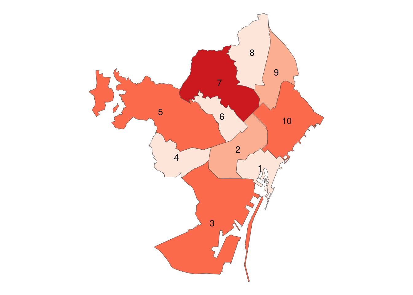

Coloring Maps with the Node Coloring Problem

Coloring maps was one of the earliest motivations to solve the node coloring problem. To color a map, we need to build a graph with nodes being the regions, connected by edges if they touch each other. As the resulting graph will be planary, we know that its chromatic number will be equal or less than four. If the map is stored as a spatial object, the connections between regions can be obtained with sf package functions.

Map coloring is a (maybe) unlikely intersection between linear programming and spatial analysis. Although we have presented a formulation that avoids symmetry, larger instances can be hard to tackle with linear programming and should be solved with other heuristics.

References

• Graph coloring instances: https://mat.tepper.cmu.edu/COLOR/instances.html
• BAdatasetsSpatial package: https://github.com/jmsallan/BAdatasetsSpatial

Session Info

## R version 4.4.1 (2024-06-14)
## Platform: x86_64-pc-linux-gnu
## Running under: Linux Mint 21.2
## 
## Matrix products: default
## BLAS:   /usr/lib/x86_64-linux-gnu/blas/libblas.so.3.10.0 
## LAPACK: /usr/lib/x86_64-linux-gnu/lapack/liblapack.so.3.10.0
## 
## locale:
##  [1] LC_CTYPE=es_ES.UTF-8       LC_NUMERIC=C              
##  [3] LC_TIME=es_ES.UTF-8        LC_COLLATE=es_ES.UTF-8    
##  [5] LC_MONETARY=es_ES.UTF-8    LC_MESSAGES=es_ES.UTF-8   
##  [7] LC_PAPER=es_ES.UTF-8       LC_NAME=C                 
##  [9] LC_ADDRESS=C               LC_TELEPHONE=C            
## [11] LC_MEASUREMENT=es_ES.UTF-8 LC_IDENTIFICATION=C       
## 
## time zone: Europe/Madrid
## tzcode source: system (glibc)
## 
## attached base packages:
## [1] stats     graphics  grDevices utils     datasets  methods   base     
## 
## other attached packages:
##  [1] ROI.plugin.glpk_1.0-0   ompr.roi_1.0.2          ompr_1.0.4             
##  [4] sf_1.0-16               BAdatasetsSpatial_0.1.0 lubridate_1.9.3        
##  [7] forcats_1.0.0           stringr_1.5.1           dplyr_1.1.4            
## [10] purrr_1.0.2             readr_2.1.5             tidyr_1.3.1            
## [13] tibble_3.2.1            ggplot2_3.5.1           tidyverse_2.0.0        
## 
## loaded via a namespace (and not attached):
##  [1] gtable_0.3.5        xfun_0.43           bslib_0.7.0        
##  [4] lattice_0.22-5      numDeriv_2016.8-1.1 tzdb_0.4.0         
##  [7] vctrs_0.6.5         tools_4.4.1         generics_0.1.3     
## [10] proxy_0.4-27        fansi_1.0.6         highr_0.10         
## [13] pkgconfig_2.0.3     Matrix_1.6-5        KernSmooth_2.23-24 
## [16] data.table_1.15.4   checkmate_2.3.1     RColorBrewer_1.1-3 
## [19] listcomp_0.4.1      lifecycle_1.0.4     farver_2.1.1       
## [22] compiler_4.4.1      munsell_0.5.1       htmltools_0.5.8.1  
## [25] class_7.3-22        sass_0.4.9          yaml_2.3.8         
## [28] lazyeval_0.2.2      pillar_1.9.0        jquerylib_0.1.4    
## [31] classInt_0.4-10     cachem_1.0.8        wk_0.9.1           
## [34] tidyselect_1.2.1    digest_0.6.35       slam_0.1-50        
## [37] stringi_1.8.3       bookdown_0.39       fastmap_1.1.1      
## [40] grid_4.4.1          colorspace_2.1-0    cli_3.6.2          
## [43] magrittr_2.0.3      utf8_1.2.4          e1071_1.7-14       
## [46] withr_3.0.0         backports_1.4.1     scales_1.3.0       
## [49] registry_0.5-1      timechange_0.3.0    rmarkdown_2.26     
## [52] blogdown_1.19       hms_1.1.3           ROI_1.0-1          
## [55] evaluate_0.23       knitr_1.46          Rglpk_0.6-4        
## [58] s2_1.1.6            rlang_1.1.4         Rcpp_1.0.12        
## [61] glue_1.7.0          DBI_1.2.2           rstudioapi_0.16.0  
## [64] jsonlite_1.8.8      R6_2.5.1            units_0.8-5