In a previous post, I presented an analysis of the Barcelona nightlife at the district level. In this post, I will make an analysis at the neighbourhood level, including:
- An assessment of which venues are inside each neighbourhood using spatial analysis.
- Evaluate the relevance of nightlife at each neighbourhood using two metrics: number of venues and venue density.
- Present choropleth maps of these metrics to examine them spatially.
I have used sf for spatial analysis. I will pick the Barcelona map through BAdatasetsSpatial. The tidyverse and kableExtra are for wrangling data, making plots and presenting nice tables.
library(tidyverse)
library(sf)
library(BAdatasetsSpatial)
library(kableExtra)
Barcelona Neighborhoods
I have retrieved the geographical information of Barcelona neighbourhoods from the map stored in BAdatasetsSPatial. I will be using the bcn_neigh map.
bcn_neigh <- BCNNeigh |>
  select(c_barri, n_barri, area, perim, coord_x, coord_y)
Barcelona is administratively divided into ten districts and seventy-three neighbourhoods. In this map, i am presenting each neighbourhood with its code.
ggplot(bcn_neigh) +
  geom_sf(fill = "white") +
  geom_text(aes(coord_x, coord_y, label = c_barri), size = 3) +
  theme_void() +
  ggtitle(label = "Barcelona Neighborhoods")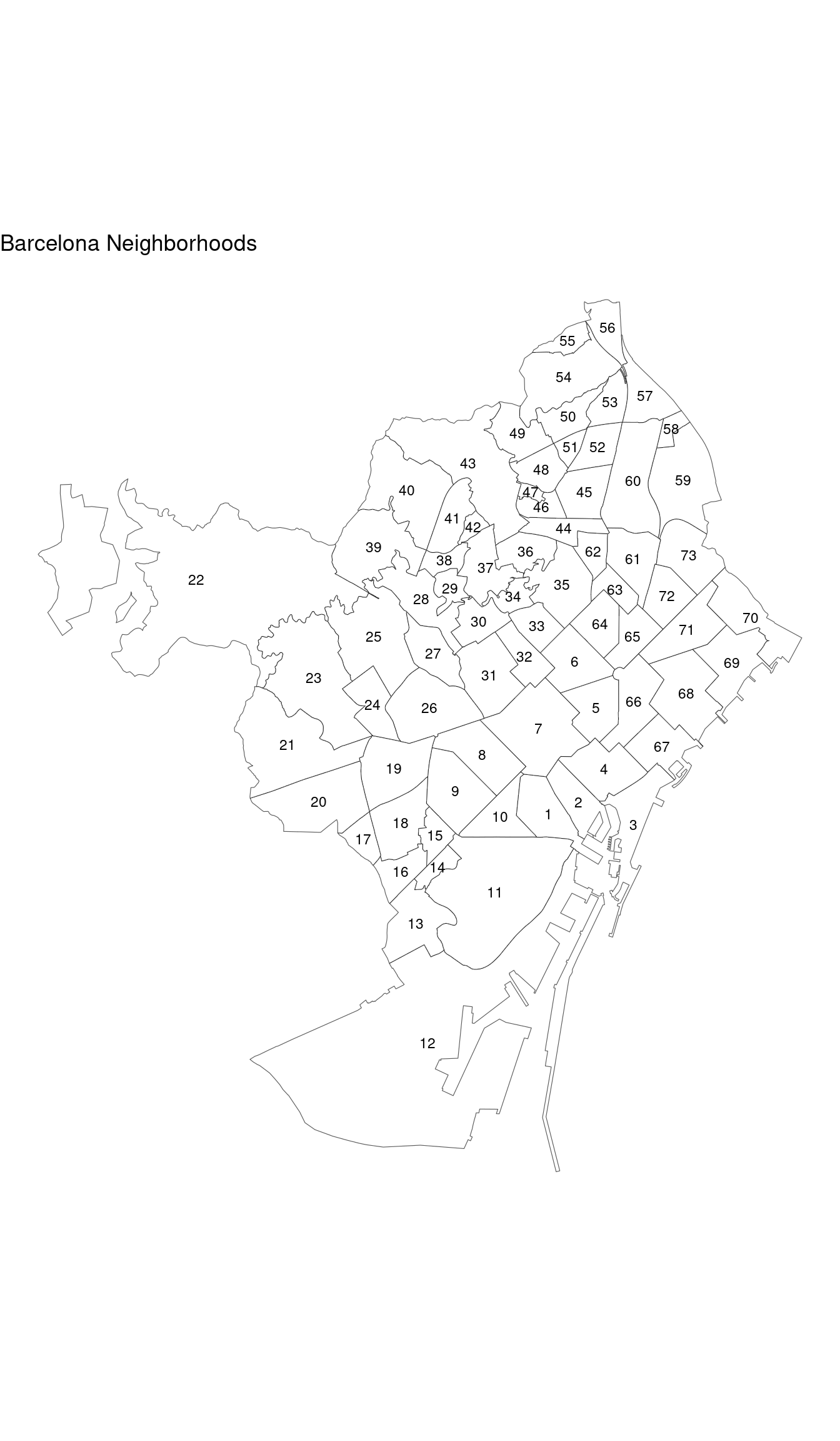
And here is the official list of neighbourhoods in Barcelona.
bcn_neigh |>
  st_drop_geometry() |>
  select(c_barri, n_barri) |>
  rename(code = c_barri, name = n_barri) |>
  arrange(code) |>
  kbl() |>
kable_minimal(full_width = FALSE)| code | name |
|---|---|
| 1 | el Raval |
| 2 | el Barri Gòtic |
| 3 | la Barceloneta |
| 4 | Sant Pere, Santa Caterina i la Ribera |
| 5 | el Fort Pienc |
| 6 | la Sagrada Família |
| 7 | la Dreta de l’Eixample |
| 8 | l’Antiga Esquerra de l’Eixample |
| 9 | la Nova Esquerra de l’Eixample |
| 10 | Sant Antoni |
| 11 | el Poble Sec |
| 12 | la Marina del Prat Vermell |
| 13 | la Marina de Port |
| 14 | la Font de la Guatlla |
| 15 | Hostafrancs |
| 16 | la Bordeta |
| 17 | Sants - Badal |
| 18 | Sants |
| 19 | les Corts |
| 20 | la Maternitat i Sant Ramon |
| 21 | Pedralbes |
| 22 | Vallvidrera, el Tibidabo i les Planes |
| 23 | Sarrià |
| 24 | les Tres Torres |
| 25 | Sant Gervasi - la Bonanova |
| 26 | Sant Gervasi - Galvany |
| 27 | el Putxet i el Farró |
| 28 | Vallcarca i els Penitents |
| 29 | el Coll |
| 30 | la Salut |
| 31 | la Vila de Gràcia |
| 32 | el Camp d’en Grassot i Gràcia Nova |
| 33 | el Baix Guinardó |
| 34 | Can Baró |
| 35 | el Guinardó |
| 36 | la Font d’en Fargues |
| 37 | el Carmel |
| 38 | la Teixonera |
| 39 | Sant Genís dels Agudells |
| 40 | Montbau |
| 41 | la Vall d’Hebron |
| 42 | la Clota |
| 43 | Horta |
| 44 | Vilapicina i la Torre Llobeta |
| 45 | Porta |
| 46 | el Turó de la Peira |
| 47 | Can Peguera |
| 48 | la Guineueta |
| 49 | Canyelles |
| 50 | les Roquetes |
| 51 | Verdun |
| 52 | la Prosperitat |
| 53 | la Trinitat Nova |
| 54 | Torre Baró |
| 55 | Ciutat Meridiana |
| 56 | Vallbona |
| 57 | la Trinitat Vella |
| 58 | Baró de Viver |
| 59 | el Bon Pastor |
| 60 | Sant Andreu |
| 61 | la Sagrera |
| 62 | el Congrés i els Indians |
| 63 | Navas |
| 64 | el Camp de l’Arpa del Clot |
| 65 | el Clot |
| 66 | el Parc i la Llacuna del Poblenou |
| 67 | la Vila Olímpica del Poblenou |
| 68 | el Poblenou |
| 69 | Diagonal Mar i el Front Marítim del Poblenou |
| 70 | el Besòs i el Maresme |
| 71 | Provençals del Poblenou |
| 72 | Sant Martí de Provençals |
| 73 | la Verneda i la Pau |
Nightlife Data
The information abouth nightlife has been retrieved from the 2024 census of ground floor premises published in Open Data BCN. As the dataset includes latitude and longitude, it can be turned into a spatial object.
nightlife_2024 <- data_2024 |>
  select(nom_local, latitud, longitud, nom_barri, codi_barri, nom_via, porta)

nightlife_2024_sf <- nightlife_2024 |>
  st_as_sf(coords = c("longitud", "latitud"), crs = 4326, remove = FALSE)

nightlife_2024_sf
## Simple feature collection with 242 features and 7 fields
## Geometry type: POINT
## Dimension: XY
## Bounding box: xmin: 2.11062 ymin: 41.37241 xmax: 2.200073 ymax: 41.43286
## Geodetic CRS: WGS 84
## # A tibble: 242 × 8
## nom_local latitud longitud nom_barri codi_barri nom_via porta
## * <chr> <dbl> <dbl> <chr> <dbl> <chr> <dbl>
## 1 LA MOLE BAR MUSICAL 41.4 2.12 Sants - … 17 TORNS 10
## 2 LA TRAVIESA TUSET 41.4 2.15 Sant Ger… 26 TUSET 10
## 3 LA CLAVE 41.4 2.13 Sants - … 17 SUGRAN… 20
## 4 PEREJIL 41.4 2.16 el Poble… 11 BLAI 10
## 5 AFTERLIFE ESPORTS GAMER … 41.4 2.14 Sant Ger… 26 MARIÀ … 10
## 6 APOLO 41.4 2.17 el Poble… 11 NOU DE… 10
## 7 APOLO BAILE 41.4 2.17 el Poble… 11 NOU DE… 20
## 8 EL GIARDINETTO 41.4 2.15 Sant Ger… 26 GRANAD… 10
## 9 APOLO CASINO 41.4 2.17 el Poble… 11 NOU DE… 50
## 10 BAR SCHULTZ 41.4 2.17 la Dreta… 7 BAILÈN 30
## # ℹ 232 more rows
## # ℹ 1 more variable: geometry <POINT [°]>Checking Data Quality
The nightlife_2024_sf includes information about the neighbourhood in the nom_barri and codi_barri columns. Let’s check if the Raval venues are located into the Raval neighbourhood. To do so, I create:
- The
nl_ravaltable of venues encoded as located at El Raval with codi_barri == 1. - The
sf_ravaltable, corresponding with the polygon of El Raval.
nl_raval <- nightlife_2024_sf |>
  filter(codi_barri == 1)

sf_raval <- bcn_neigh |>
  filter(c_barri == 1)
Let’s plot both spatial objects together.
ggplot(sf_raval) +
  geom_sf() +
  geom_sf(data = nl_raval)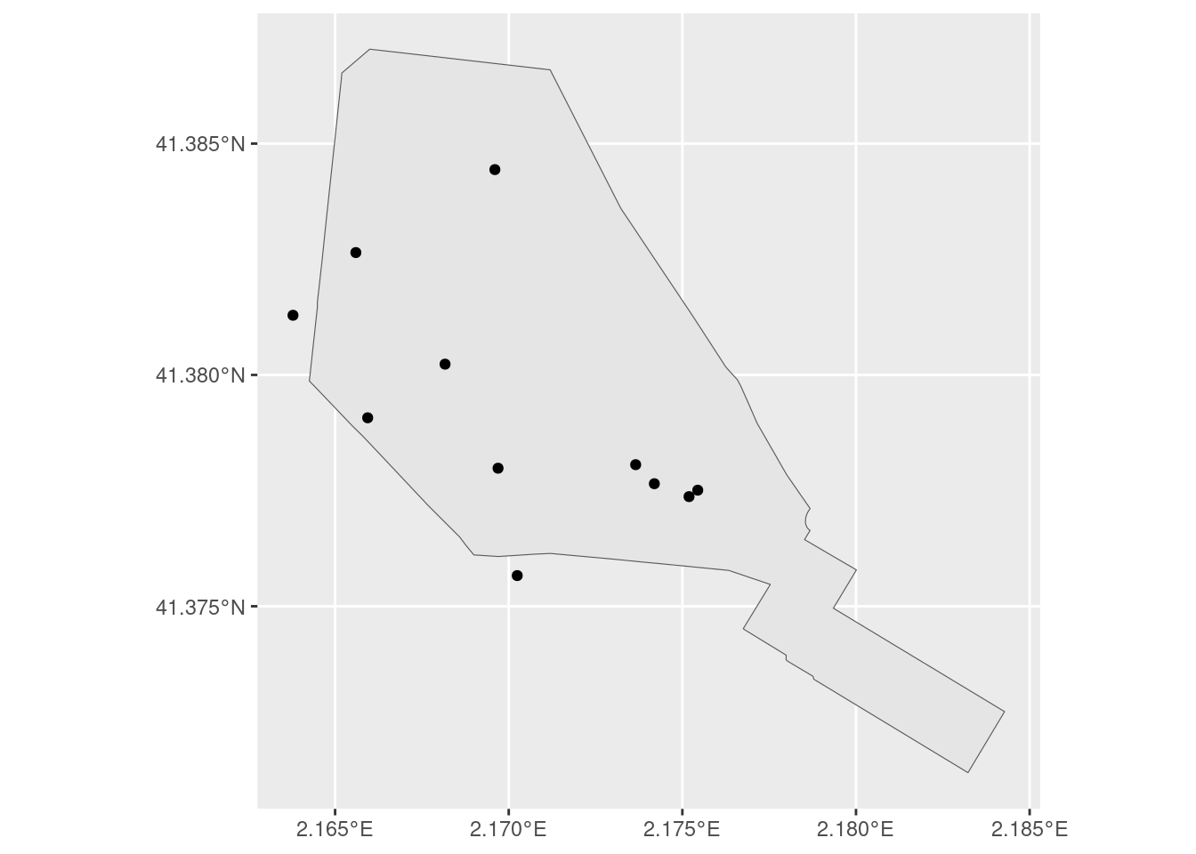
Some of the points fall outside the polygon (and maybe there are points inside the polygon incorrectly encoded too). We need to assign points to neighborhoods spatially using sf::st_join(). The result is stored in nightlife_2024_sf2.
nightlife_2024_sf2 <- st_join(nightlife_2024_sf,
                              bcn_neigh |> select(c_barri, n_barri),
                              join = st_intersects)
In one case the spatial join has not found the neighborhood, so we keep it in the original neighborhood.
nightlife_2024_sf2 <- nightlife_2024_sf2 |>
  mutate(c_barri = ifelse(is.na(c_barri), codi_barri, c_barri),
         n_barri = ifelse(is.na(c_barri), nom_barri, n_barri))
The neighbourhood code assigned spatially is in c_barri and the code included in the nightlife dataset is in codi_barri. We can appreciate some differences:
nightlife_2024_sf2 |>
  filter(c_barri != codi_barri)
## Simple feature collection with 43 features and 9 fields
## Geometry type: POINT
## Dimension: XY
## Bounding box: xmin: 2.127625 ymin: 41.37542 xmax: 2.195337 ymax: 41.43224
## Geodetic CRS: WGS 84
## # A tibble: 43 × 10
## nom_local latitud longitud nom_barri codi_barri nom_via porta
## * <chr> <dbl> <dbl> <chr> <dbl> <chr> <dbl>
## 1 ALIMENTACIÓ MONK 41.4 2.18 Sant Pere,… 4 ABAIXA… 10
## 2 BLING BLING 41.4 2.15 Sant Gerva… 26 TUSET 20
## 3 RATAFIA 41.4 2.13 les Tres T… 24 RAFAEL… 20
## 4 ARENA XPERIENCE 41.4 2.17 la Dreta d… 7 RDA SA… 40
## 5 EL PATRÓN SHISHA LOUNGE 41.4 2.14 el Putxet … 27 MANUEL… 10
## 6 ARENA CHICAS 41.4 2.16 la Dreta d… 7 DIPUTA… 20
## 7 IMPERATOR 41.4 2.16 la Vila de… 31 CÒRSEGA 10
## 8 SALA VIVALDI 41.4 2.15 Sant Antoni 10 LLANÇA 10
## 9 BEACH CLUB 41.4 2.15 l'Antiga E… 8 VALÈNC… 10
## 10 SCOBIE'S IRISH PUB 41.4 2.17 la Dreta d… 7 RDA UN… 20
## # ℹ 33 more rows
## # ℹ 3 more variables: geometry <POINT [°]>, c_barri <dbl>, n_barri <chr>Let’s check where are the points assigned to c_barri == 1.
nl2_raval <- nightlife_2024_sf2 |>
  filter(c_barri == 1)

ggplot(sf_raval) +
  geom_sf() +
  geom_sf(data = nl2_raval)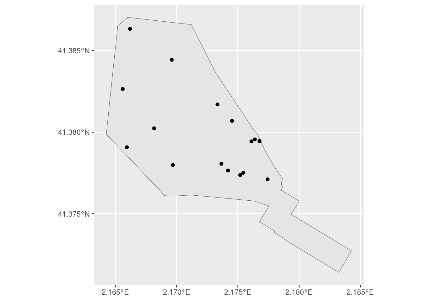
Seeing the results, I will be using the c_barri column to assign venues to neighbourhoods.
Metrics of Neighborhood Nightlife
I will be using two metrics to evaluate the intensity of nightlife in a neighbourhood:
- Number of venues.
- Venue density, measured in number of venues per square kilometer.
These metrics will be stored in the count_nl table. I am grouping by c_barri and count to obtain venues per neighbourhood.
count_nl <- nightlife_2024_sf2 |>
  st_drop_geometry() |>
  group_by(c_barri) |>
  summarise(venues = n(), .groups = "drop")
count_nl
## # A tibble: 35 × 2
## c_barri venues
## <dbl> <int>
## 1 1 16
## 2 2 23
## 3 3 3
## 4 4 16
## 5 5 3
## 6 6 1
## 7 7 14
## 8 8 11
## 9 9 8
## 10 10 7
## # ℹ 25 more rowsSeeing the number of rows of count_nl, not all neighbourhoods have nightlife. I will pick the area of the incumbent neighbourhoods from bcn_neigh making a left_join() with count_nl as first table.
count_nl <- left_join(count_nl,
                      bcn_neigh |>
                        st_drop_geometry() |>
                        select(c_barri, n_barri, area),
                      by = "c_barri")
As the area is in square meters, I transform it in square kilometers and then compute density.
count_nl <- count_nl |>
  mutate(area = area/1e+06,
         density = venues/area)
The ten neighbourhoods with more nightlife venues are:
count_nl |>
  arrange(-venues) |>
  select(n_barri, venues, density) |>
  slice(1:10) |>
  kbl() |>
kable_styling(full_width = FALSE)| n_barri | venues | density |
|---|---|---|
| Sant Gervasi - Galvany | 32 | 19.289704 |
| el Barri Gòtic | 23 | 27.318994 |
| el Poble Sec | 23 | 4.995069 |
| el Raval | 16 | 14.566736 |
| Sant Pere, Santa Caterina i la Ribera | 16 | 14.358806 |
| la Vila de Gràcia | 15 | 11.312043 |
| la Dreta de l’Eixample | 14 | 6.593185 |
| l’Antiga Esquerra de l’Eixample | 11 | 8.910827 |
| les Corts | 11 | 7.787210 |
| Sants | 9 | 8.198509 |
And the top ten neighbourhoods by venue density of venues:
count_nl |>
  arrange(-density) |>
  select(n_barri, venues, density) |>
  slice(1:10) |>
  kbl() |>
kable_styling(full_width = FALSE)| n_barri | venues | density |
|---|---|---|
| el Barri Gòtic | 23 | 27.318994 |
| Sant Gervasi - Galvany | 32 | 19.289704 |
| el Raval | 16 | 14.566736 |
| Sant Pere, Santa Caterina i la Ribera | 16 | 14.358806 |
| la Vila de Gràcia | 15 | 11.312043 |
| l’Antiga Esquerra de l’Eixample | 11 | 8.910827 |
| Sant Antoni | 7 | 8.739239 |
| Sants | 9 | 8.198509 |
| les Corts | 11 | 7.787210 |
| Sants - Badal | 3 | 7.307104 |
Choropleth Maps
I will present the results of above as choroplet maps. I need to add the values of count_nl to bcn_neigh. As we need to keep all the regions of the map, I use a left_join() with bcn_neigh as first table.
bcn_neigh <- left_join(bcn_neigh,
                       count_nl |>
                         select(c_barri, venues, density),
                       by = "c_barri")
Some neighborhoods have no venues, so I replace NA by zeros in venues and density.
bcn_neigh <- bcn_neigh |>
  mutate(venues= ifelse(is.na(venues), 0, venues),
         density = ifelse(is.na(density), 0, density))
Now I can do the choropleth of the number of venues. I have chosen a gradient fill color scale with low value white (for neighbourhoods with no venues) to red (maximum value of venues).
ggplot(bcn_neigh) +
  geom_sf(aes(fill = venues)) +
  scale_fill_gradient(low = "white", high = "red") +
  theme_void() +
  theme(legend.position = "none") +
  labs(title = "Number of Venues by Neighborhood (2024)",
          caption = "Source: Open Data BCN")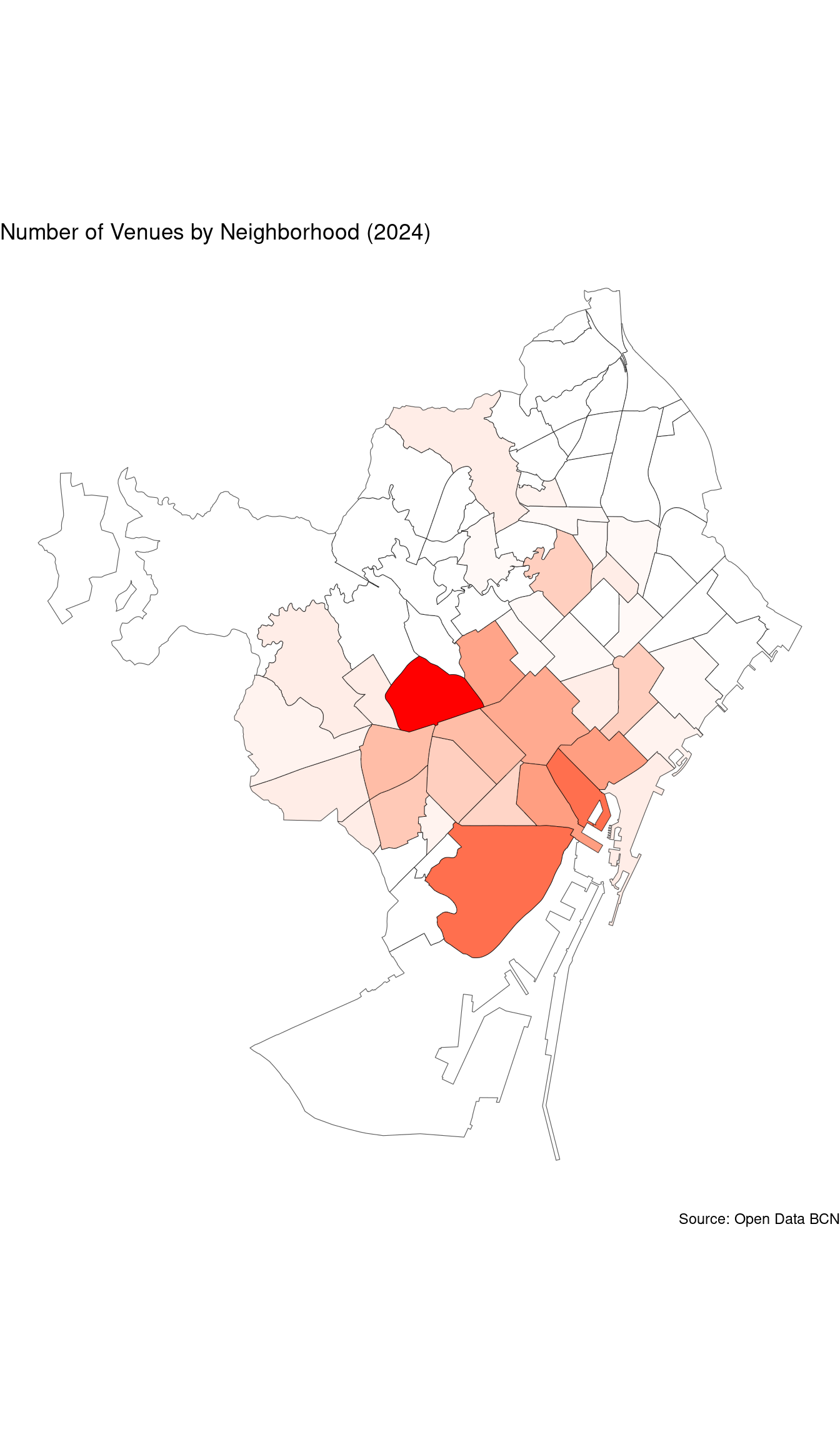
The venue density choropleth is built with the same principle, using orange instead of red.
ggplot(bcn_neigh) +
  geom_sf(aes(fill = density)) +
  scale_fill_gradient(low = "white", high = "orange") +
  theme_void() +
  theme(legend.position = "none") +
  labs(title = "Venue Density by Neighborhood (2024)",
          caption = "Source: Open Data BCN")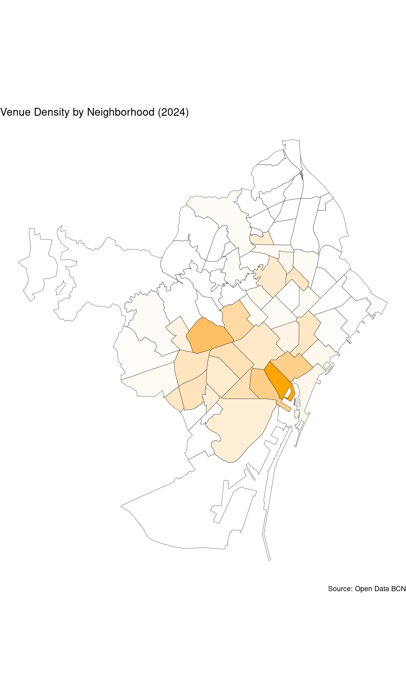
Conclusions
In this post, I have used a Barcelona neighbourhood map to analyze the intensity of nightlife across the city. I have used a spatial join to assign a neighbourhood to each venue, and I have calculated two metrics: the number of venues and density of venues for each neighbourhood. I have used this information to present a top ten ranking of neighbourhoods and a choropleth for each metric.
Results show two distinct geographical zones: the residential neighbourhood of Sant Gervasi-Galvany and downtown neighbourhoods. Public of Sant Gervasi–Galvany is predominantly middle- to upper-middle-class residents. Many patrons are locals from the district or nearby upscale areas (Sarrià, Tres Torres, Eixample). Nightlife here tends to be more oriented toward cocktail bars, lounges, and premium venues. The public of downtonw neighbourhoods like Barri Gòtic, El Raval, Poble Sec and Sant Pere, Santa Caterina i la Ribera is more socially mixed but heavily influenced by tourists, visitors, and young people from across the city. There is presence of international residents, students, and creative communities. In the Barri Gòtic especially, the nightlife public is tourism-driven, with a high proportion of short-term visitors.
References
- Census of premises on the ground floor intended for economic activity in the city of Barcelona https://opendata-ajuntament.barcelona.cat/data/en/dataset/cens-locals-planta-baixa-act-economica.
Session Info
## R version 4.5.2 (2025-10-31)
## Platform: x86_64-pc-linux-gnu
## Running under: Linux Mint 21.1
##
## Matrix products: default
## BLAS:   /usr/lib/x86_64-linux-gnu/blas/libblas.so.3.10.0
## LAPACK: /usr/lib/x86_64-linux-gnu/lapack/liblapack.so.3.10.0  LAPACK version 3.10.0
##
## locale:
##  [1] LC_CTYPE=es_ES.UTF-8       LC_NUMERIC=C
##  [3] LC_TIME=es_ES.UTF-8        LC_COLLATE=es_ES.UTF-8
##  [5] LC_MONETARY=es_ES.UTF-8    LC_MESSAGES=es_ES.UTF-8
##  [7] LC_PAPER=es_ES.UTF-8       LC_NAME=C
##  [9] LC_ADDRESS=C               LC_TELEPHONE=C
## [11] LC_MEASUREMENT=es_ES.UTF-8 LC_IDENTIFICATION=C
##
## time zone: Europe/Madrid
## tzcode source: system (glibc)
##
## attached base packages:
## [1] stats     graphics  grDevices utils     datasets  methods   base
##
## other attached packages:
##  [1] kableExtra_1.4.0        BAdatasetsSpatial_0.1.0 sf_1.0-20
##  [4] lubridate_1.9.4         forcats_1.0.1           stringr_1.6.0
##  [7] dplyr_1.1.4             purrr_1.2.0             readr_2.1.5
## [10] tidyr_1.3.1             tibble_3.3.0            ggplot2_4.0.0
## [13] tidyverse_2.0.0
##
## loaded via a namespace (and not attached):
##  [1] s2_1.1.7           utf8_1.2.4         sass_0.4.10        generics_0.1.3
##  [5] xml2_1.4.1         class_7.3-23       KernSmooth_2.23-26 blogdown_1.21
##  [9] stringi_1.8.7      hms_1.1.4          digest_0.6.37      magrittr_2.0.4
## [13] evaluate_1.0.3     grid_4.5.2         timechange_0.3.0   RColorBrewer_1.1-3
## [17] bookdown_0.43      fastmap_1.2.0      jsonlite_2.0.0     e1071_1.7-16
## [21] DBI_1.2.3          viridisLite_0.4.2  scales_1.4.0       textshaping_1.0.0
## [25] jquerylib_0.1.4    cli_3.6.4          rlang_1.1.6        units_0.8-7
## [29] withr_3.0.2        cachem_1.1.0       yaml_2.3.10        tools_4.5.2
## [33] tzdb_0.5.0         vctrs_0.6.5        R6_2.6.1           proxy_0.4-27
## [37] lifecycle_1.0.4    classInt_0.4-11    pkgconfig_2.0.3    pillar_1.11.1
## [41] bslib_0.9.0        gtable_0.3.6       Rcpp_1.1.0         glue_1.8.0
## [45] systemfonts_1.2.3  xfun_0.52          tidyselect_1.2.1   rstudioapi_0.17.1
## [49] knitr_1.50         farver_2.1.2       htmltools_0.5.8.1  labeling_0.4.3
## [53] svglite_2.2.0      rmarkdown_2.29     wk_0.9.4           compiler_4.5.2
## [57] S7_0.2.0