Analysis of necessity

Social phenomena may depend on many complex causal configurations, although some may be more important than others. Necessary conditions are those without which the outcome cannot occur. Baumoller and Goetz (2000) established that \(X\) is a necessary condition of \(Y\) if:

• \(X\) is always present when \(Y\) occurs,
• \(Y\) does not occur in the absence of \(X\).

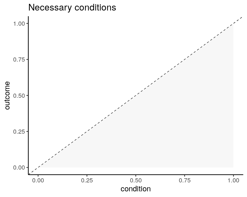
In terms of set theory, set \(X\) is a necessary condition of set \(Y\) if \(Y\) is a subset of \(X\).

We represent the necessity relationship as \(X \Leftarrow Y\)

Let’s examine which variables are necessary conditions of the outcome SURV in the crisp version of the Lipset dataset LC. To do so, we examine the cases included in set SURV:

LC %>% filter(SURV == 1)

##    DEV URB LIT IND STB SURV
## BE   1   1   1   1   1    1
## CZ   1   1   1   1   1    1
## FI   1   0   1   0   1    1
## FR   1   0   1   1   1    1
## IE   1   0   1   0   1    1
## NL   1   1   1   1   1    1
## SE   1   0   1   1   1    1
## UK   1   1   1   1   1    1

We observe that all elements of set SURV are also included in sets DEV, LIT and STB. So, these are necessary conditions for SURV to happen. The reverse implication does not hold: for instance, if we pick all cases where DEV occurs we observe that two of them to SURV.

LC %>% select(DEV, SURV) %>% filter(DEV == 1)

##    DEV SURV
## AU   1    0
## BE   1    1
## CZ   1    1
## FI   1    1
## FR   1    1
## DE   1    0
## IE   1    1
## NL   1    1
## SE   1    1
## UK   1    1

With fuzzy sets, the condition of necessity that \(Y\) is a subset of \(X\) means that if \(X\) is a necessary condition of \(Y\), fuzzy scores of \(X\) are higher than fuzzy scores of \(Y\). If we plot fuzzy memberships of \(Y\) versus fuzzy memberships of \(X\), cases of necessary conditions will appear in the lower area of the plot:

In real datasets, a condition is rarely a perfect necessary condition. We examine the extent to which a condition is necessary with consistency and coverage.

The consistency or inclusion of a necessary condition is the extent to which \(X\) is a necessary condition of \(Y\). In fuzzy sets it is defined as:

\[inc\left(X \Leftarrow Y \right) = \frac{ \sum min\left(X,Y\right)}{\sum Y}\]

A value of consistency close to one means that \(X\) is close to be a necessary condition for \(Y\): inclusion only is present when consistency is equal to one. In the LC dataset, DEV, LIT and STB have values of consistency equal to one.

\(X\) may be a necessary condition of \(Y\), but it can happen that many members of \(X\) do not belong to \(Y\). To account for this, we define coverage for fuzzy sets as:

\[cov\left(X \Leftarrow Y \right) = \frac{ \sum min\left(X,Y\right)}{\sum X}\]

A coverage close to one means that most of the elements of set \(X\) are also included in set \(Y\). In the sample LC the set DEV has ten elements, of which eight belong to set SURV: the coverage for DEV is 0.8. A high coverage for a necessary condition shows that it is a relevant one to explain the outcome.

If all or most of all the elements of the sample belong to the set \(X\), it is very likely that \(X\) be a necessary condition of any outcome, but a trivial one. For instance, air is necessary for fire, but we always have air available so air can be considered a trivial condition for fire. To account for this, Schneider and Wagemann (2012) defined the relevance of a necessary condition as:

\[rel\left(X \Leftarrow Y \right) = \frac{ \sum \left(1-X\right)}{\sum \left( 1- min\left(X,Y\right)\right)}\]

An example of non-relevant condition for the LC crisp dataset is the LIT variable:

LC %>% select(LIT, SURV) %>% filter(LIT == 1)

##    LIT SURV
## AU   1    0
## BE   1    1
## CZ   1    1
## EE   1    0
## FI   1    1
## FR   1    1
## DE   1    0
## HU   1    0
## IE   1    1
## NL   1    1
## PL   1    0
## SE   1    1
## UK   1    1

Thirteen out of eighteen cases of the dataset are included in LIT. As a consequence, its relevance is of 0.5 and it can be considered as a condition of low relevance. .

We can obtain consistency, coverage and relevance for specific conditions with the pof function. setms is a data frame with columns with the conditions or a sum of products expression, and data is the dataset with the scores. Here we are assessing the fuzzy-set dataset LF:

pof(setms = LF %>% select(-SURV),  outcome = "SURV", data = LF, relation = "necessity")

## 
##         inclN   RoN   covN  
## --------------------------- 
## 1  DEV  0.831  0.811  0.775 
## 2  URB  0.539  0.899  0.771 
## 3  LIT  0.991  0.509  0.643 
## 4  IND  0.669  0.786  0.684 
## 5  STB  0.920  0.680  0.707 
## ---------------------------

We can achieve the same using a sum of products expression:

pof(setms = "DEV+URB+LIT+IND+STB", outcome = "SURV", data = LF, relation = "necessity")

## 
##                inclN   RoN   covN  
## ---------------------------------- 
## 1         DEV  0.831  0.811  0.775 
## 2         URB  0.539  0.899  0.771 
## 3         LIT  0.991  0.509  0.643 
## 4         IND  0.669  0.786  0.684 
## 5         STB  0.920  0.680  0.707 
## 6  expression  1.000  0.357  0.583 
## ----------------------------------

In the last row we obtain the parameters for the whole logical expression. Values of inclusion appear on the inclN column, relevance on RoN and coverage on covN.

In the following plots, I am comparing the fuzzy scores of SURV with three variables:

• DEV: a condition with high consistency, relevance and coverage.
• LIT: a condition with high consistency, but low relevance.
• URB: a condition with low consistency.

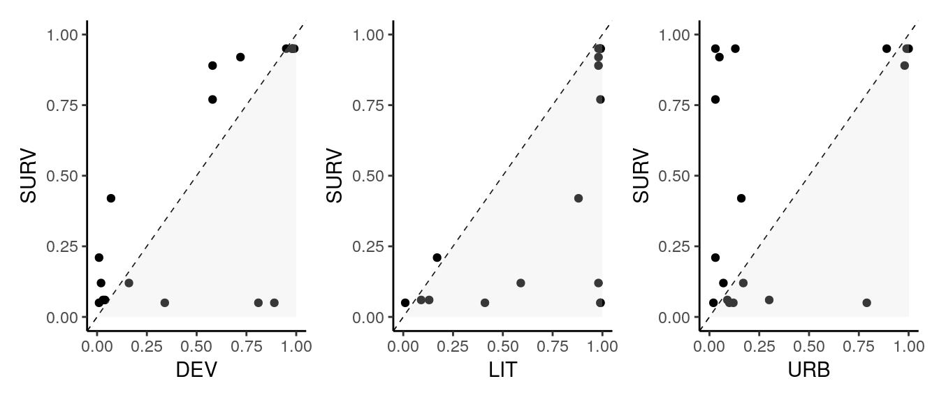
Note that as scores of \(X\) should be higher than scores of \(Y\), most of the cases must be in the lower triangle for a necessary condition to be consistent. This is what is happening with DEV and LIT, but not with URB. In the LIT plot, we observe that many cases have an score near to one: that’s why LIT has less relevance than DEV.

We can do an analysis of necessity with logical expressions presented in a sum of products format, where the product * stands for the AND logical operator (set intersection) and the sum + for the OR operator (set union). We can negate variables using the ~ symbol.

pof(setms = "DEV*~LIT+IND*STB", outcome = "SURV", data = LF, relation = "necessity")

## 
##                inclN   RoN   covN  
## ---------------------------------- 
## 1    DEV*~LIT  0.045  0.984  0.567 
## 2     IND*STB  0.664  0.873  0.783 
## 3  expression  0.670  0.872  0.784 
## ----------------------------------

Here we have examined necessity relations of original explanatory variables, but we might want to explore possible necessity relations of all possible sums of products. We can do that with the superSubset function. It explores all possible necessity relationships, and present those with minimum values of consistency, coverage or relevance. Here I have retained conditions with consistency higher than 0.8 and relevance higher than 0.7.

superSubset(LF, "SURV", incl.cut = 0.9, ron.cut = 0.7)

## 
##                 inclN   RoN   covN  
## ----------------------------------- 
## 1  LIT*STB      0.915  0.800  0.793 
## 2  DEV+URB+IND  0.903  0.704  0.716 
## -----------------------------------

Analysis of sufficiency

The aim of the analysis of sufficiency is to find the minimal configurations that are sufficient to obtain the outcome set. The formal definition of sufficiency is structurally similar to necessity. We say that \(X\) is a sufficient condition for \(Y\) when:

• every time \(X\) is present, \(Y\) is present.
• \(X\) does not occur in the absence of \(Y\).

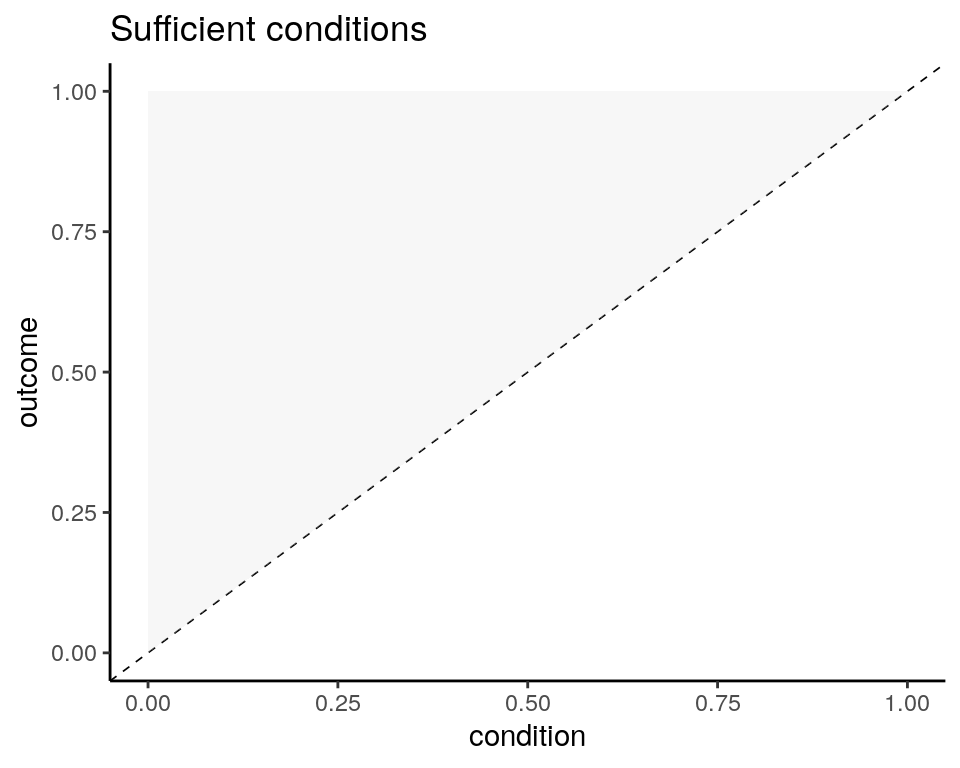
In terms of set theory, \(X\) is a sufficient condition for \(Y\) if \(X\) is a subset of \(Y\). When applying fuzzy logic, the fuzzy scores of \(Y\) must be higher than the ones of \(X\). For perfect sufficiency, all cases must be in the upper triangle of the \(\left(X,Y\righ)\) plot.

We can define the consistency or inclusion of a sufficient relationship as:

\[inc\left(X \Rightarrow Y \right) = \frac{ \sum min\left(X,Y\right)}{\sum X}\]

A perfect sufficient relationship will have a consistency score of one. The smaller the consistency, the further is the condition for being sufficient to obtain the outcome.

In some cases, we find that a condition can be sufficient to explain the outcome and the negated outcome, examining consistency and coverage alone. To illustrate this, we can use data from Dușa (2021):

pri_test <- data.frame(X = c(0.2, 0.4, 0.45, 0.5, 0.6),
Y = c(0.3, 0.5, 0.55, 0.6, 0.7))

Let’s examine the sufficiency of \(X\) for $Y and for \(\sim Y\):

pof(pri_test %>% select(X), "Y", pri_test, relation = "sufficiency")

## 
##        inclS   PRI   covS   covU  
## --------------------------------- 
## 1   X  1.000  1.000  0.811    -   
## ---------------------------------

pof(pri_test %>% select(X), "~Y", pri_test, relation = "sufficiency")

## 
##        inclS   PRI   covS   covU  
## --------------------------------- 
## 1   X  0.814  0.000  0.745    -   
## ---------------------------------

For both outcomes we observe good values of consistence and coverage for sufficiency, but we cannot make a condition sufficient for the outcome and its negation. To help to choose between the two outcomes Ragin (2006) defines the proportional reduction of inconsistency (PRI) rate as:

\[ PRI = \frac{ \sum min\left(X,Y\right) - \sum min\left( X, Y, \sim Y \right)}{\sum X - \sum min\left( X, Y, \sim Y \right)} \]

We assign the condition to the outcome with the largest PRI, in this case \(Y\) rather than \(\sim Y\).

The concept of sufficiency allows for more than one sufficient condition to explain the outcome. That’s why QCA is particularly suitable to analyze situations of equifinality, where an outcome can be obtained in different ways. In the context of sufficiency, raw coverage measures how much of the outcome Y is explained by a condition X:

\[cov\left(X \Rightarrow Y \right) = \frac{ \sum min\left(X,Y\right)}{\sum Y}\]

If we have obtained more than one set of sufficient conditions \(A, B, C, \dots\), some cases might belong to more than one condition. We may be interested in finding how much a condition alone explains the outcome in this context. This is measured by the unique coverage, measured as:

\[ covU\left(A \Rightarrow Y \right) = \frac{\sum min\left(A,Y\right) - \sum min\left(A,Y, max\left(B, C, \dots \right)\right)}{\sum Y} \]

A typical task of a sufficient condition analysis is to find all the sufficient conditions. This task is carried out in two steps:

• Assign a value of outcome to existing combinations of observable variables through a truth table.
• Simplify the conditions where the outcome is observed with a minimization process using the Quine-McCluskey algorithm.

Bibliography and resources

• Braumoeller, B. and Goertz, G. (2000). The Methodology of Necessary Conditions. American Journal of Political Science, 44 (4):844–858. https://doi.org/10.2307/2669285^.
• Dușa, Adrian (2021). QCA with R: A Comprehensive Resource. https://bookdown.org/dusadrian/QCAbook/
• Lipset, S. M. (1959). Some Social Requisites of Democracy: Economic Development and Political Legitimacy. American Political Science Review, 53:69-105.
• Ragin, C. C. (2006). User’s Guide to Fuzzy-Set/Qualitative Comparative Analysis 2.0. Tucson, Arizona: Department of Sociology, University of Arizona.
• Schneider, C. and Wagemann, C. (2012). Set-Theoretic Methods for the Social Sciences. A Guide to Qualitative Comparative Analysis. Cambridge: Cambridge University Press.

Built with R 4.1.1, patchwork 1.1.1, QCA 3.12 and tidyverse 1.3.1