Motifs in Undirected Networks

Jose M Sallan 2025-05-31 12 min read

Complex network analysis usually examines networks at the global level, with metrics like average path length, average clustering coefficient and global and local efficiency. They are also examined at the local level, with measures such as node degree or node and edge betweenness.

In complex networks theory, there is a stream of reseearch focusing on intermediate network structures obtained from the examination of subgraphs. A subgraph is a subset of a graph, sharing some or all of its nodes and edges. The analysis of subgraphs allows us to identify network motifs. Motifs are patterns of interconnections of a network, occurring at a number significantly higher than in randomized versions of the graph: a random graph with the same number of nodes, edges and degree distribution.

In this post, I will introduce how to use the R igraph library to identify network motifs. These network motifs can be described as isomorphism classes of subgraphs (usually between three and finve nodes) more abundant than in a random network. I will also use purrr for functional programming and data.table for tabular data handling.

library(igraph)
library(purrr)
library(data.table)

Isomorphic Classes of Subgraphs

Two graphs are isomorphic when there is a matching between nodes of each graph so that two nodes connected in the first graph correspond to nodes connected in the second graph. A set of isomorphic graphs forms an isomorphic class. To be isomorphic, graphs need to have the same number of nodes, so it is frequent to consider isomorphic classes for a given number of nodes. Let’s illustrate this with two isomorphic graphs of four nodes.

g1 <- graph_from_literal(A -- B, B -- D, C -- D, C -- A)
g1 <- permute(g1, c(1, 2, 4, 3))
g2 <- graph_from_literal(A -- D, D -- B, B -- C, C -- A)
g2 <- permute(g2, c(1, 4, 2, 3))

layout4 <- matrix(c(0, 1,
                    1, 1,
                    0, 0,
                    1, 0), nrow = 4, byrow = TRUE)

iso4 <- list(g1, g2)

par(mfrow = c(1, 2), oma = c(0.5, 1, 0.5, 1), mar = c(1, 1, 1, 1))
walk(iso4, ~ plot(., vertex.size = 40, vertex.color = "white", layout = layout4))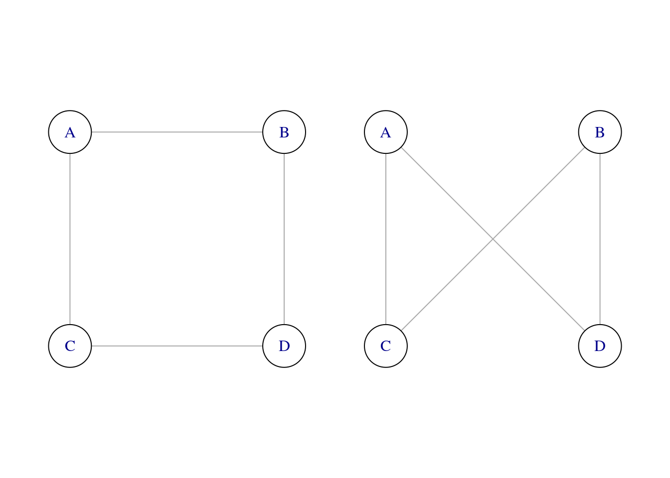

If subgraphs of the same isomorphic classe appear in a network at an abnormal rate, they are be considered a motif of that network. To examine subgraphs, we have several functions in igraph:

motifs(g, n) counts the subgraphs of each isomorphic class of size n (number of nodes) in a graph g.
count_motifs(g, n) returns the total number of subgraphs of size n in g.

To illustrate this, let’s consider a power grid network:

power_grid

## IGRAPH f3f2e8d UN-- 4941 6594 -- 
## + attr: id (v/c), name (v/c)
## + edges from f3f2e8d (vertex names):
##  [1] 6 --8   7 --8   8 --9   9 --10  5 --13  12--13  13--14  13--15  14--16 
## [10] 14--17  18--19  19--20  14--29  33--34  34--35  35--36  36--37  36--38 
## [19] 36--39  41--42  36--47  44--47  45--47  46--47  10--50  21--51  24--53 
## [28] 25--58  41--58  58--59  59--60  9 --61  31--62  63--68  64--68  65--68 
## [37] 35--69  66--69  68--69  67--70  69--70  72--73  9 --75  48--75  76--77 
## [46] 78--79  79--80  81--82  13--83  71--86  76--86  4 --88  55--88  87--88 
## [55] 87--89  88--90  73--91  11--94  26--94  43--94  92--94  93--94  94--95 
## [64] 34--97  40--97  28--98  42--98  57--98  74--98  82--98  98--100 99--100
## + ... omitted several edges

Let’s apply the two functions to power_grid for subgraphs of size n = 3 nodes.

motifs(power_grid, 3) # four motifs of size 3

## [1]    NA    NA 16980   651

count_motifs(power_grid, 3)    # total number of motifs of a given size in igraph

## [1] 17631

As seen in motifs() each isomorphism class has a number, corresponding to its classification in igraph. To find a representative of a isomorphism class, we have the function graph_from_isomorphism_class(). From the result of motifs() we have learned that there are four isomorphism classes of size three. These are labelled from zero to three. Let’s obtain each of the representatives:

graph3_list <- map(0:3, ~ graph_from_isomorphism_class(3, ., directed = FALSE))
titles3 <- paste0("isomorphism ", 0:3)

Let’s define a layout for a graph of three nodes.

layout3 <- matrix(c(0, 2,
                    1, 1,
                    0, 0), nrow = 3, byrow = TRUE)

And here are each of the representatives of each of the isomorphic classes of size three.

par(mfrow = c(2, 2), oma = c(0.5, 1, 0.5, 1), mar = c(1, 1, 1, 1))
walk2(graph3_list, titles3, ~ plot(.x, vertex.size = 40, vertex.color = "white", layout = layout3, main = .y))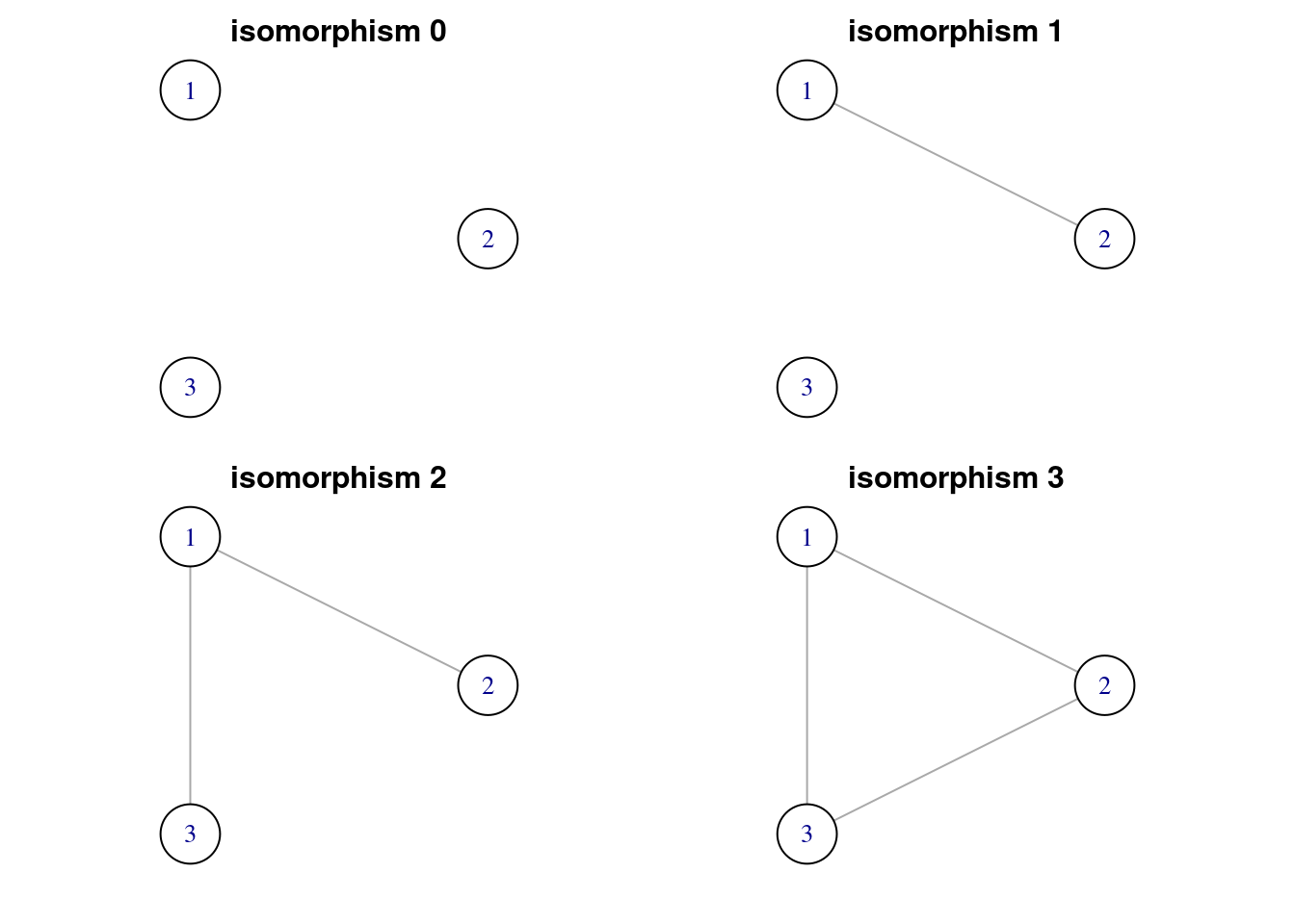

When we have applied the motifs() function to the graph, some of the results are NA. These correspond to unconnected graphs that are not considered as candidates to motifs of order three. Then the possible motifs of order three are:

motifs3_list <- graph3_list[which(!is.na(motifs(power_grid, 3)))]
titles_motifs3 <- titles3[which(!is.na(motifs(power_grid, 3)))]

par(mfrow = c(1, 2), oma = c(0.5, 1, 0.5, 1), mar = c(1, 1, 1, 1))
walk2(motifs3_list, titles_motifs3, ~ plot(.x, vertex.size = 40, vertex.color = "white", layout = layout3, main = .y))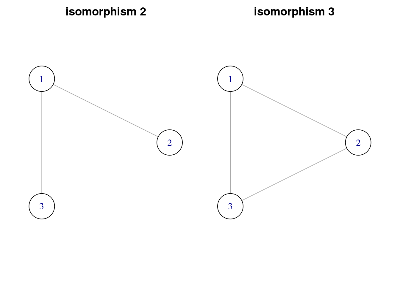

We can repeat the same workflow to obtain the eleven isomorphic classes of size four. Let’s start counting motifs of the sample graph.

motifs(power_grid, 4)

##  [1]    NA    NA    NA    NA 19826    NA 37682  5094   324   385    90

There are eleven isomorphic classes:

graph4_list <- map(0:10, ~ graph_from_isomorphism_class(4, ., directed = FALSE))
numbers4 <- substr(as.character(100:110), 2, 3)
titles4 <- paste0("isomorphism ", numbers4)

layout4 <- matrix(c(0, 1,
                    1, 1,
                    0, 0,
                    1, 0), nrow = 4, byrow = TRUE)

par(mfrow = c(4, 3), oma = c(0.5, 1, 0.5, 1), mar = c(1, 1, 1, 1))
walk2(graph4_list, titles4, ~ plot(.x, vertex.size = 40, vertex.color = "white", layout = layout4, main = .y))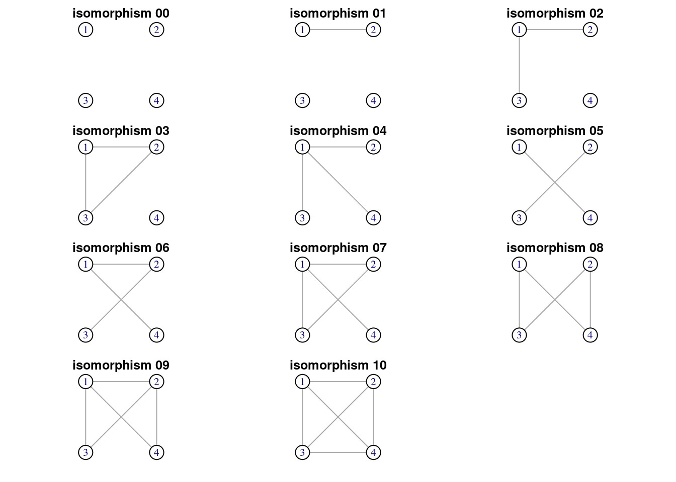

Of the eleven isomorphic classes, only six correspond to possible network motifs.

motifs4_list <- graph4_list[which(!is.na(motifs(power_grid, 4)))]
titles_motifs4 <- titles4[which(!is.na(motifs(power_grid, 4)))]

par(mfrow = c(2, 3), oma = c(0.5, 1, 0.5, 1), mar = c(1, 1, 1, 1))
walk2(motifs4_list, titles_motifs4, ~ plot(.x, vertex.size = 40, vertex.color = "white", layout = layout4, main = .y))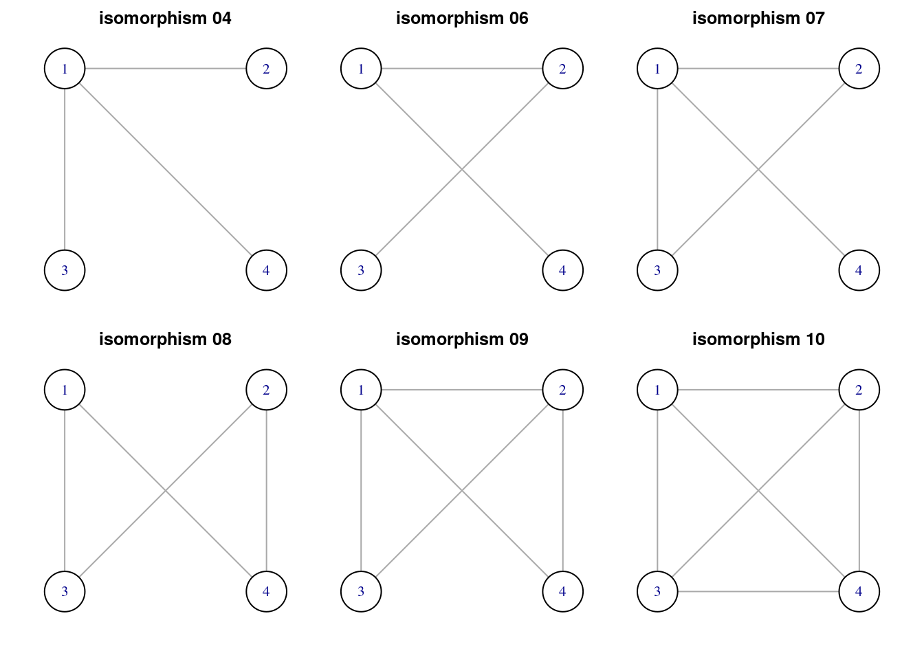

Let’s count the isomorphic classes of size five.

motifs(power_grid, 5)

##  [1]     NA     NA     NA     NA     NA     NA     NA     NA     NA     NA
## [11]     NA  25101     NA 118571   8616  82780  12036   3171   1926     NA
## [21]  11703   1785    785     23    107    818    311    355    315     30
## [31]    215      8     23     15

There are 34 isomorphic classes of size five, of which 21 are considered connected and then candidates to motifs. Let’s plot the possible motifs of size five.

graph5_list <- map(0:33, ~ graph_from_isomorphism_class(5, ., directed = FALSE))
numbers5 <- substr(as.character(100:133), 2, 3)
titles5 <- paste0("isomorphism ", numbers5)

m5 <- which(!is.na(motifs(power_grid, 5)))

motifs5_list <- graph5_list[m5]
titles_motifs5 <- titles5[m5]

layout5 <- matrix(c(cos(2*pi*0:4/5 + pi/2), 
                    sin(2*pi*0:4/5 + pi/2)), nrow = 5)

par(mfrow = c(7, 3), oma = c(0.5, 1, 0.5, 1), mar = c(1, 1, 1, 1))
walk2(motifs5_list, titles_motifs5, ~ {plot(.x, 
                                    vertex.size = 40, vertex.color = "white", 
                                    layout = layout5)
  title(.y, cex.main = 0.8)})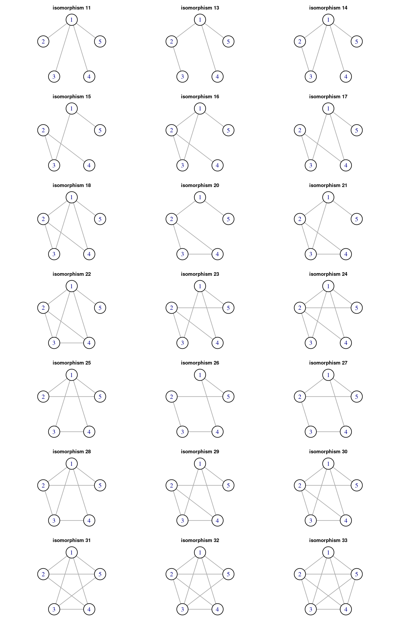

For undirected graphs, igraph goes as far as subgraphs of size six:

motifs(power_grid, 6)

##   [1]     NA     NA     NA     NA     NA     NA     NA     NA     NA     NA
##  [11]     NA     NA     NA     NA     NA     NA     NA     NA     NA     NA
##  [21]     NA     NA     NA     NA     NA     NA     NA     NA     NA     NA
##  [31]     NA     NA     NA     NA  33749     NA 179144  12571     NA  86407
##  [41] 257075  38765   5498   3077     NA  19350   2541    983   4440   2224
##  [51]     NA     NA 241372   8020     NA  35826 180917   6734  53371   7820
##  [61]   2078   2225    132    416   2450   3530   1592    698  26523   7312
##  [71]   1601   1411    125    814     NA   6964    138     NA   4384    630
##  [81]    738    124   4273   1448    879     19     72     63    128     NA
##  [91]   2053    601    115    132      1     35    558    571     63     73
## [101]     24    170      0     59    331    356    175     27     76    275
## [111]     88     14     49    152      4     22      1     18      0     30
## [121]     NA   2000    826    177    188     73    299     27     61    137
## [131]    180     25     11     49     48      0     49      0      1      0
## [141]      0      2     26      0      6      9     10      0     12      2
## [151]      1     13      0      0      0      2

We have up to 156 subgraphs of size six, of which which(!is.na(motifs(power_grid, 6))) |> length() are considered motifs.

Table with Isomorphic Classes

To count all isomorphic classes of subgraphs available in igraph, I have defined the motif_count() function. It takes a graph g as argument and returns a data table with all subgraphs of size n belonging to isomorphic class m.

motif_count <- function(g){
  
  motif_count <- map_dfr(3:6, ~ {
    mc <- motifs(g, .)
    df <- data.table(n = ., m = 0:(length(mc) - 1), mc = mc)
    df <- df[!is.na(mc)]
  })
  
  return(motif_count)
}

This is the result of applying the function to the power grid:

motif_count(power_grid)

##          n     m    mc
##      <int> <int> <num>
##   1:     3     2 16980
##   2:     3     3   651
##   3:     4     4 19826
##   4:     4     6 37682
##   5:     4     7  5094
##  ---                  
## 137:     6   151    13
## 138:     6   152     0
## 139:     6   153     0
## 140:     6   154     0
## 141:     6   155     2

Detecting Motifs in a Graph

To detect the motifs of the power grid, we need to compare the frequency of each subgraph with the one of random graphs with the same number of nodes, edges and degree sequence. The later is obtained with degree().

degree_pg <- degree(power_grid)

We can generate random graphs with a fixed degree sequence with the sample_degseq() function. I am using using the Viger and Latapy method passing method = "vl".

set.seed(55)
sample_degseq(degree_pg, method = "vl")

## IGRAPH f6b8f59 U--- 4941 6594 -- Degree sequence random graph
## + attr: name (g/c), method (g/c)
## + edges from f6b8f59:
##  [1]  1--1017  1--1502  1--2461  2--3785  2--2982  2--  10  2--2822  3--2881
##  [9]  4-- 790  5-- 545  6--4405  6--1624  7--1105  8--3926  9--3227  9--3873
## [17]  9--2198 10--3956 10-- 638 10--1311 10-- 338 10-- 795 11--3839 11-- 670
## [25] 12-- 637 12-- 216 13--1334 14--4861 14--3828 14--3774 14--2844 14--3187
## [33] 15--4591 15--1270 15--3085 15--4148 15--1981 16--4479 17--1050 18--4436
## [41] 19--2315 19--2329 20-- 142 20--2675 20--1952 21--2393 21--1194 22--4873
## [49] 22--3526 23--2535 24--1290 25--2940 25--1045 26--1392 26--3602 27-- 817
## [57] 27--4795 27--2802 27--3838 28--1202 28--1469 29-- 131 30--2503 30--1879
## + ... omitted several edges

To detect network motifs, I am using the method described in Milo et al. (2002) and Milo et al. (2004). From a sample of random graphs with the same degree sequence we obtain the average and standard deviation of the number of appearances of each motif $N_{i}^{r a n d}$ . Then, I compute the z-score for motif $i$ :

$z_{i} = \frac{N_{i}^{r e a l} - ⟨ N_{i}^{r a n d} ⟩}{s d (N_{i}^{r a n d})}$

Where $⟨ N_{i}^{r a n d} ⟩$ and $s d (N_{i}^{r a n d})$ are the mean and the standard deviation of number of motifs $i$ , respectively. As $N_{i}^{r a n d}$ is normally distributed, network motifs will have values of $z_{i}$ above the upper significance threshold. We can also speak of antimotifs, with values of $z_{i}$ below than the lower significance threshold. Antimotifs are subgraphs that appear with a lesser frequence than in an equivalent random network.

To perform this test I have written the motif_detector() function. In addition to the graph g, takes as arguments:

sample_size: the number of random graphs to be evaluated.
sig_level: the level of significance to detect motifs and antimotifs.

motif_detector <- function(g, sample_size, sig_level = 0.01){
  
  degseq <- degree(g)
  
  # sampling motifs
  random_sg <- map_dfr(1:sample_size, ~{
    # random sample graph
    rs <- sample_degseq(degseq, method = "vl")
    mc <- motif_count(rs)
  })
  rt <- random_sg[, .(mean = mean(mc), sd = sd(mc)), .(n, m)]
  
  # motifs of g
  rn <- motif_count(g)
  setnames(rn, "mc", "mc_real")
  
  # merging and computing z score
  md <- merge(rt, rn, by = c("n", "m"))
  md[, z := (mc_real - mean)/sd]
  
  # significance thresholds
  lt <- qnorm(sig_level)
  ut <- qnorm(1 - sig_level)
  md[, motif := "no motif"]
  md[z < lt, motif := "antimotif"]
  md[z > ut, motif := "motif"]
  
  return(md)
  
}

Motifs of the Power Grid Network

Let’s apply this function to the power grid network:

mpg <- motif_detector(power_grid, sample_size = 1000)

Let’s examine motifs of size three:

mpg[n == 3]

## Clave <n, m>
##        n     m      mean       sd mc_real         z     motif
##    <int> <int>     <num>    <num>   <num>     <num>    <char>
## 1:     3     2 18921.849 5.851704   16980 -331.8433 antimotif
## 2:     3     3     3.717 1.950568     651  331.8433     motif

The closed triangle (n = 3, m = 3) is a motif of this network.

mpg[n == 4]

## Clave <n, m>
##        n     m      mean         sd mc_real          z     motif
##    <int> <int>     <num>      <num>   <num>      <num>    <char>
## 1:     4     4 26003.758  26.440774   19826 -233.64512 antimotif
## 2:     4     6 53233.384 522.243674   37682  -29.77802 antimotif
## 3:     4     7    46.204  26.394792    5094  191.24212     motif
## 4:     4     8     7.807   2.829798     324  111.73694     motif
## 5:     4     9     0.019   0.136593     385 2818.45261     motif
## 6:     4    10     0.000   0.000000      90        Inf     motif

Higher-order isomorphic classes are motifs of this network. This suggests that this network has more clustered regions than a random network of similar degree distribution.

References

Graph motifs (igraph R manual): https://igraph.org/r/doc/motifs.html
Graph isomorphism: https://www2.math.upenn.edu/~mlazar/math170/notes05-2.pdf
Milo, R., Itzkovitz, S., Kashtan, N., Levitt, R., Shen-Orr, S., Ayzenshtat, I., … & Alon, U. (2004). Superfamilies of evolved and designed networks. Science, 303(5663), 1538-1542.
Milo, R., Shen-Orr, S., Itzkovitz, S., Kashtan, N., Chklovskii, D., & Alon, U. (2002). Network motifs: simple building blocks of complex networks. Science, 298(5594), 824-827.

Session Info

## R version 4.5.0 (2025-04-11)
## Platform: x86_64-pc-linux-gnu
## Running under: Linux Mint 21.1
## 
## Matrix products: default
## BLAS:   /usr/lib/x86_64-linux-gnu/blas/libblas.so.3.10.0 
## LAPACK: /usr/lib/x86_64-linux-gnu/lapack/liblapack.so.3.10.0  LAPACK version 3.10.0
## 
## locale:
##  [1] LC_CTYPE=es_ES.UTF-8       LC_NUMERIC=C              
##  [3] LC_TIME=es_ES.UTF-8        LC_COLLATE=es_ES.UTF-8    
##  [5] LC_MONETARY=es_ES.UTF-8    LC_MESSAGES=es_ES.UTF-8   
##  [7] LC_PAPER=es_ES.UTF-8       LC_NAME=C                 
##  [9] LC_ADDRESS=C               LC_TELEPHONE=C            
## [11] LC_MEASUREMENT=es_ES.UTF-8 LC_IDENTIFICATION=C       
## 
## time zone: Europe/Madrid
## tzcode source: system (glibc)
## 
## attached base packages:
## [1] stats     graphics  grDevices utils     datasets  methods   base     
## 
## other attached packages:
## [1] data.table_1.17.0 purrr_1.0.4       igraph_2.1.4     
## 
## loaded via a namespace (and not attached):
##  [1] vctrs_0.6.5       cli_3.6.4         knitr_1.50        rlang_1.1.6      
##  [5] xfun_0.52         generics_0.1.3    jsonlite_2.0.0    glue_1.8.0       
##  [9] htmltools_0.5.8.1 sass_0.4.10       rmarkdown_2.29    tibble_3.2.1     
## [13] evaluate_1.0.3    jquerylib_0.1.4   fastmap_1.2.0     yaml_2.3.10      
## [17] lifecycle_1.0.4   bookdown_0.43     compiler_4.5.0    dplyr_1.1.4      
## [21] pkgconfig_2.0.3   rstudioapi_0.17.1 blogdown_1.21     digest_0.6.37    
## [25] R6_2.6.1          tidyselect_1.2.1  pillar_1.10.2     magrittr_2.0.3   
## [29] bslib_0.9.0       tools_4.5.0       cachem_1.1.0

The Jose M Sallan static website