In this post, I will introduce the moderation relationship in linear regression. After defining moderation, I am presenting two examples with a categorical and continuous moderating variables, respectively. I am taking advantage of the possiblities of the tidyverse to plot interactions with ggplot, and to define a function to compute simple slopes using dplyr programmatically. Finally, I brielfy introduce the interactions package to visualize interactions in linear regression.
A moderator \(z\) is a variable that affects the direction and/or strength of the relationship between an independent variable \(x\) and a dependent variable \(y\). We often express this relationship in terms of interaction between \(x\) and \(z\) respect to its relationship with \(y\). In van Vegchel et al. (2005) we can find several possible modelisations of variable interaction.
The most common modelisation of moderation is to assume a linear evolution of the influence of the moderating variable. This linear interaction occurs when the regression coefficient of the product of dependent and moderator is significant.
\[\begin{align} y &= \beta_0 + \left( \beta_1 + \beta_2z \right) + \varepsilon \\ y &= \beta_0 + \beta_1x + \beta_2xz + \varepsilon \end{align}\]
The most common way of estimating a linear moderation effect is through moderated multiple regression (Aguinis & Gottfredson, 2010):
\[\begin{align} y &= \beta_0 + \beta_1x + \beta_2z + \beta_3xz + \varepsilon \end{align}\]
To confirm the existence of a moderating variable, we need to check if the regression coefficient of the product (interaction) term \(\beta_3\) is significant. Note that in this model the distinction between dependent and moderating variable is theoretical, as ariables \(x\) and \(z\) are treated similarly.
The moderated multiple regression model can be called from R using a formula like y ~ x * z in the lm function call. This syntax generates regression variables x, z and x:z, the later representing the interaction term. If we wanted to enter the interaction term alone, we just specify a formula like y ~ x:z.
The workflow of the moderation analysis is slightly different depending if the moderator is categorical or continuous. Let’s examine an example of each.
Categorical moderator
We will use the mtcars dataset, that includes fuel consumption and 10 aspects of automobile design and performance for 32 automobiles (1973–74 models). My hypothesis is that the influence of weight wt on fuel consumption mpg in miles per gallon is moderated by the categorical variable type of transmission am (0 = automatic, 1 = manual).
Let’s build the moderated multiple regression model:
mt_model <- lm(mpg ~ wt * am, mtcars)Let’s examine the summary of mt_model:
summary(mt_model)##
## Call:
## lm(formula = mpg ~ wt * am, data = mtcars)
##
## Residuals:
## Min 1Q Median 3Q Max
## -3.6004 -1.5446 -0.5325 0.9012 6.0909
##
## Coefficients:
## Estimate Std. Error t value Pr(>|t|)
## (Intercept) 31.4161 3.0201 10.402 4.00e-11 ***
## wt -3.7859 0.7856 -4.819 4.55e-05 ***
## am 14.8784 4.2640 3.489 0.00162 **
## wt:am -5.2984 1.4447 -3.667 0.00102 **
## ---
## Signif. codes: 0 '***' 0.001 '**' 0.01 '*' 0.05 '.' 0.1 ' ' 1
##
## Residual standard error: 2.591 on 28 degrees of freedom
## Multiple R-squared: 0.833, Adjusted R-squared: 0.8151
## F-statistic: 46.57 on 3 and 28 DF, p-value: 5.209e-11The interaction term wt:am is significant, so we can assert that am moderates the relationship between wt and mpg. I have chosen am as moderator instead of wt on theoretical grounds alone, as the moderated multiple regression model treats both variables equally.
To observe how the interaction works, we can examine the effect of wt on mpg for the two values of am using ggplot:
ggplot(mtcars, aes(wt, mpg, color = factor(am))) +
  geom_point() +
  geom_smooth(method = "lm", se = FALSE) +
  scale_color_manual(name = "transmission", labels = c("automatic", "manual"), values = c("#FF6666", "#6666FF")) +
  theme_classic()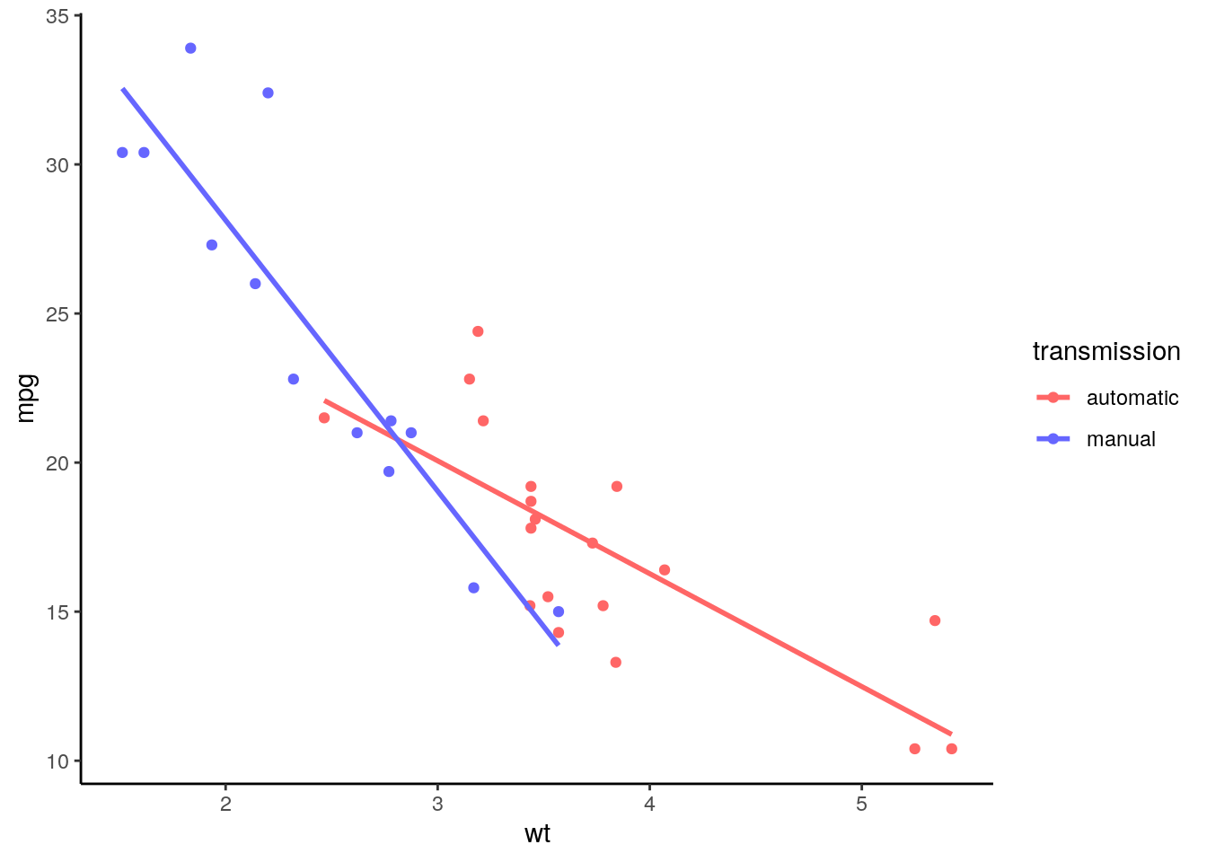
This plot allows us to see how it is the relationship between dependent and independent variables for each value of the categorical moderator. Fuel consumption always increases with weight, but this increase is higher for cars with manual transmission than for cars with automatic transmission. We learn this because the slope for manual transmission is steeper than for automatic transmission.
Continuous moderator
To examine how to deal with a continuous moderator, we will use the depress dataset, obtained from Zhang and Wang (2016-2020):
depress <- read.csv("depress.csv")
head(depress)
## stress support depress
## 1 7 5 32
## 2 8 7 20
## 3 2 2 30
## 4 7 6 25
## 5 6 9 19
## 6 2 8 25The theoretical guess made by authors is that the influence of stress on depression depress is moderated by social support. Let’s examine the results of the moderated multiple regression model.
depress_model <- lm(depress ~ support * stress, depress)
summary(depress_model)
##
## Call:
## lm(formula = depress ~ support * stress, data = depress)
##
## Residuals:
## Min 1Q Median 3Q Max
## -3.7322 -0.9035 -0.1127 0.8542 3.6089
##
## Coefficients:
## Estimate Std. Error t value Pr(>|t|)
## (Intercept) 29.2583 0.6909 42.351 <2e-16 ***
## support -0.2356 0.1109 -2.125 0.0362 *
## stress 1.9956 0.1161 17.185 <2e-16 ***
## support:stress -0.3902 0.0188 -20.754 <2e-16 ***
## ---
## Signif. codes: 0 '***' 0.001 '**' 0.01 '*' 0.05 '.' 0.1 ' ' 1
##
## Residual standard error: 1.39 on 96 degrees of freedom
## Multiple R-squared: 0.9638, Adjusted R-squared: 0.9627
## F-statistic: 853 on 3 and 96 DF, p-value: < 2.2e-16We observe that the interaction term support:stress is significant. To know how is the effect of the moderator on the relationship between the dependent and independent variables, we use simple slopes plots. These plots present the relationship between dependent and independent variable for three subsets of data:
- Observations with high values of the moderator \(z > \bar{z} + s_z\).
- Observations with low values of the moderator \(z < \bar{z} - s_z\).
- The rest of medium values of the moderator.
I have defined a simple_slopes function, taking as inputs the dataset and character strings with the names of dependent, independent and moderator variables.
simple_slopes <- function(data, dependent, independent, moderator){

  dataset <- data %>% select(.data[[dependent]], .data[[independent]], .data[[moderator]])
  names(dataset) <- c("dep", "ind", "mod")

  sd_mod <- sd(dataset$mod)
  mean_mod <- mean(dataset$mod)

  dataset <- dataset %>%
    mutate(level_mod = case_when(mod < mean_mod - sd_mod ~ "low",
                                mod > mean_mod + sd_mod ~ "high",
                                TRUE ~ "medium")) %>%
    mutate(level_mod = factor(level_mod, levels = c("high", "medium", "low")))

  plot <- ggplot(dataset, aes(ind, dep, color = level_mod)) +
    geom_point() +
    geom_smooth(method = "lm", se = FALSE) +
    scale_color_manual(name = moderator, values = c("#336600", "#66CC00", "#B2FF66")) +
    labs(x = independent, y = dependent) +
    theme_bw()

  return(plot)

}
The result of applying the function to the dataset is:
simple_slopes(depress, "depress", "stress", "support")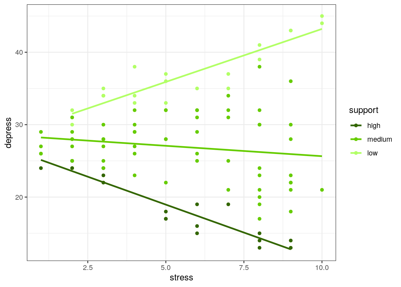
The simple slopes plot tells us a complex moderating relationship. For high values of support, the relationship between stress and depression is negative, while the relationship is positive for low values of social support.
The interactions package
Instead of the function above, we can use the interactions package (Long, 2021).
library(interactions)The function interact_plot produces simple slopes plots by specifying the model and the names of the dependent and moderating variables:
interact_plot(depress_model, "stress", "support", plot.points = TRUE)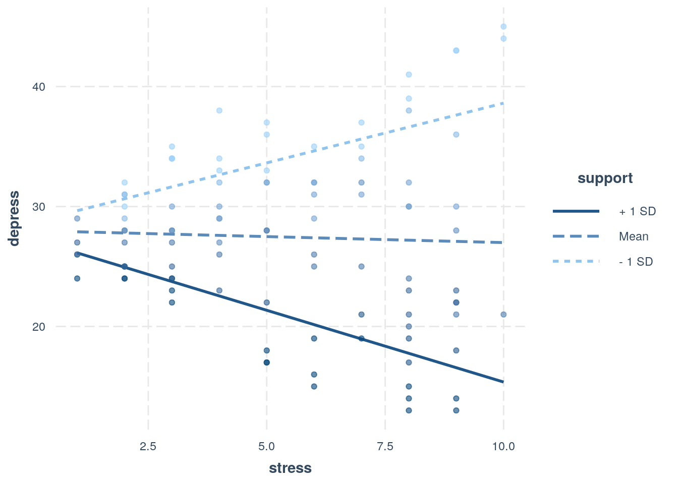
The package also works with categorical moderators:
interact_plot(mt_model, wt, am, plot.points = TRUE)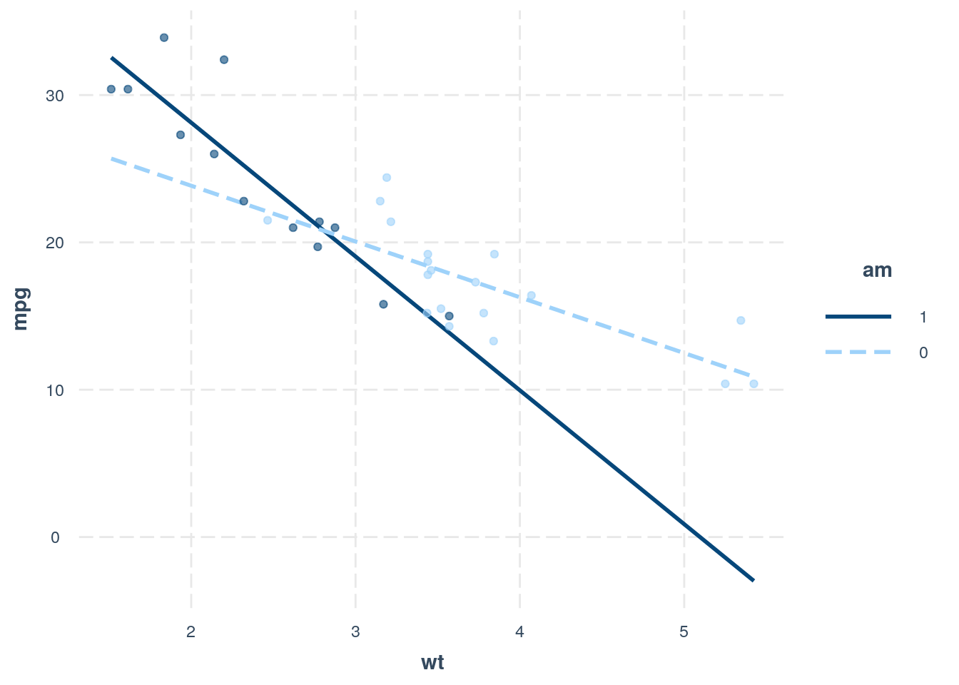
In Long (2021) can be found other functionalities of this package, designed to visualize interactions between variables in linear regression.
References
- Aguinis, H., & Gottfredson, R. K. (2010). Best-practice recommendations for estimating interaction effects using moderated multiple regression. Journal of Organizational Behavior, 31(6), 776–786. https://doi.org/10.1002/job.686
- Baron, R. M., & Kenny, D. A. (1986). The moderator-mediator variable distinction in social psychological research: conceptual, strategic, and statistical considerations. Journal of Personality and Social Psychology, 51(6), 1173–1182. Retrieved from http://www.ncbi.nlm.nih.gov/pubmed/3806354
- Long, J. (2021). Exploring interactions with continuous predictors in regression models. https://cran.r-project.org/web/packages/interactions/vignettes/interactions.html
- Programming with dplyr https://cran.r-project.org/web/packages/dplyr/vignettes/programming.html
- van Vegchel, N., de Jonge, J., & Landsbergis, P. a. (2005). Occupational stress in (inter)action: the interplay between job demands and job resources. Journal of Organizational Behavior, 26(5), 535–560. https://doi.org/10.1002/job.327
- Zhang, Z. & Lijuan Wang, L. (2016-2020). Moderation analysis, in Advanced statistics using R. https://advstats.psychstat.org/book/moderation/index.php
Session info
## R version 4.1.2 (2021-11-01)
## Platform: x86_64-pc-linux-gnu (64-bit)
## Running under: Debian GNU/Linux 10 (buster)
##
## Matrix products: default
## BLAS:   /usr/lib/x86_64-linux-gnu/blas/libblas.so.3.8.0
## LAPACK: /usr/lib/x86_64-linux-gnu/lapack/liblapack.so.3.8.0
##
## locale:
##  [1] LC_CTYPE=es_ES.UTF-8       LC_NUMERIC=C
##  [3] LC_TIME=es_ES.UTF-8        LC_COLLATE=es_ES.UTF-8
##  [5] LC_MONETARY=es_ES.UTF-8    LC_MESSAGES=es_ES.UTF-8
##  [7] LC_PAPER=es_ES.UTF-8       LC_NAME=C
##  [9] LC_ADDRESS=C               LC_TELEPHONE=C
## [11] LC_MEASUREMENT=es_ES.UTF-8 LC_IDENTIFICATION=C
##
## attached base packages:
## [1] stats     graphics  grDevices utils     datasets  methods   base
##
## other attached packages:
##  [1] interactions_1.1.5 forcats_0.5.1      stringr_1.4.0      dplyr_1.0.7
##  [5] purrr_0.3.4        readr_2.0.2        tidyr_1.1.4        tibble_3.1.5
##  [9] ggplot2_3.3.5      tidyverse_1.3.1
##
## loaded via a namespace (and not attached):
##  [1] Rcpp_1.0.6        lubridate_1.8.0   lattice_0.20-45   assertthat_0.2.1
##  [5] digest_0.6.27     utf8_1.2.1        R6_2.5.0          cellranger_1.1.0
##  [9] backports_1.2.1   reprex_2.0.1      evaluate_0.14     highr_0.9
## [13] httr_1.4.2        blogdown_1.5      pillar_1.6.4      rlang_0.4.12
## [17] readxl_1.3.1      rstudioapi_0.13   jquerylib_0.1.4   Matrix_1.3-4
## [21] rmarkdown_2.9     labeling_0.4.2    splines_4.1.2     pander_0.6.4
## [25] munsell_0.5.0     broom_0.7.10      compiler_4.1.2    modelr_0.1.8
## [29] xfun_0.23         pkgconfig_2.0.3   mgcv_1.8-38       htmltools_0.5.1.1
## [33] tidyselect_1.1.1  bookdown_0.24     fansi_0.5.0       crayon_1.4.1
## [37] tzdb_0.1.2        dbplyr_2.1.1      withr_2.4.2       grid_4.1.2
## [41] nlme_3.1-153      jsonlite_1.7.2    gtable_0.3.0      lifecycle_1.0.0
## [45] DBI_1.1.1         magrittr_2.0.1    scales_1.1.1      cli_3.0.1
## [49] stringi_1.7.3     farver_2.1.0      fs_1.5.0          xml2_1.3.2
## [53] bslib_0.2.5.1     jtools_2.1.4      ellipsis_0.3.2    generics_0.1.0
## [57] vctrs_0.3.8       tools_4.1.2       glue_1.4.2        hms_1.1.1
## [61] yaml_2.2.1        colorspace_2.0-1  rvest_1.0.2       knitr_1.33
## [65] haven_2.4.3       sass_0.4.0