A common problem of statistics is to make inferences about the parameters of a probability distribution. By inference, or statistical inference, we mean to deduce properties of a population from a sample. A example of inference is to estimate the mean height of the inhabitants of a country from a sample or subset of individuals of that country.
To make statistical inferences, we need to make assumptions about the joint probability distribution of the observations. This joint probability distribution is the probability to observe a sample given fixed values of the parameters of the distribution. Following with the mean height example, the central limit theorem asserts that the mean of the height of a sample of individuals picked randomly follows a normal distribution, with mean equal to the population mean. So we make the assumption that the sample mean follows a normal distribution.
When we make statistical inferences, we have a fixed set of observations, and our job is to obtain estimators of the parameters. Then we turn the joint probability distribution into a likelihood function. The likelihood function is the probability of some estimated values of the parameters, given fixed values of the random variables. We often consider that the maximum likelihood estimates of the parameters are the best values we can choose in statistical inference.
Maximum likelihood estimates of a binomial event
Let’s suppose that we have a population of red and white balls, and that a ball is red with an unknown probability \(p\). This \(p\) is the parameter of a binomial probability distribution, that gives us the probability that \(k\) out of \(n\) balls are red as:
\[ P\left[ \left( n, k \right), p \right] = \binom{n}{k} p^k \left( 1 - p \right)^\left( n-k \right) \]
Let’s suppose now that we take 5 balls from the population, and that two are red and three white. We are observing that \(n=5\) and \(k=2\), so the likelihood function for this population is:
\[ \mathcal{L} \left[ p, \left( 5, 2 \right) \right] = \binom{5}{2} p^2 \left( 1 - p \right)^3 \]
The value of \(p\) that maximizes \(\mathcal{L} \left( p \right)\) will be the maximum likelihood estimator of the probability of the population. Let’s represent the likelihood function:
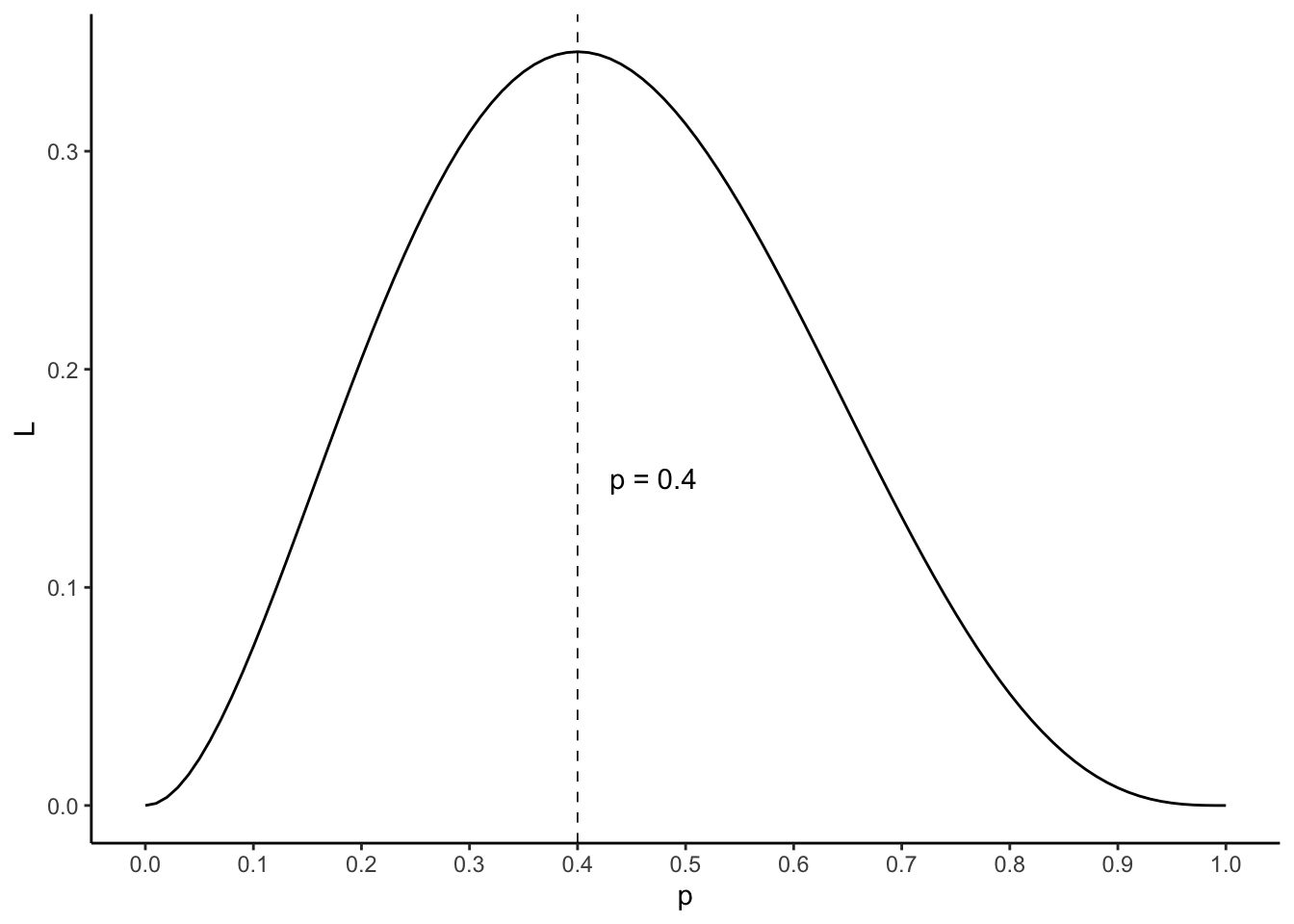
It is likely that you are not surprised when you learn that the maximum likelihood estimator of \(p\) is \(2/5 = 0.4\).
Maximum likelihood estimates of a normal distribution
Let’s suppose now that we have a sample of \(n\) independent observations \(\mathbf{x} = \left\{ x_1, \dots, x_n \right\}\) from a normal distribution with un{kown population mean \(\mu\) and population variance \(\sigma^2\). The density probability function of this variable is the Gaussian function:
\[ P \left( x, \left( \mu, \sigma \right) \right) = \frac{1}{\sigma \sqrt{2\pi}} \text{exp}\left[ - \frac{\left( x - \mu \right)^2}{2 \sigma^2} \right] \]
If the observations of \(\mathbf{x}\) are independent and coming from the same normal distribution \(N\left( \mu, \sigma \right)\), the probability of joint ocurrrence is equal to the product of the values of the Gaussian function for each observation. Then, we can define the likelihood function as:
\[ \mathcal{L} \left[ \left( \mu, \sigma \right), \mathbf{x} \right] = \prod_{i=1}^n \frac{1}{\sigma \sqrt{2\pi}} \text{exp}\left[ - \frac{\left( x_i - \mu \right)^2}{2 \sigma^2} \right] \]
Finding the minimum of this function can be hard. A way of making this easier is to minimize the logarithm of the likelihood function. This arises frequently when we are dealing with likelihood functions with normal distributions, and it is known as log likelihood function \(\mathcal{l} \left[ \left( \mu, \sigma \right), \mathbf{x} \right]\). We can use the log likelihood instead of the likelihood because the logarithm is a monotonous function.
The log of the above likelihood function is:
\[ \mathcal{l} \left[ \left( \mu, \sigma \right), \mathbf{x} \right] = - \frac{n}{2}ln\left( 2\pi \right) - \frac{n}{2}ln \left( \sigma^2 \right) - \frac{1}{2 \sigma^2} \sum_{i=1}^n \left( x_i - \mu \right)^2 \]
To obtain the maximum likelihood estimates of mean and variance \(\hat{mu}\) we equal to zero the partial derivative:
\[ \frac{\partial \mathcal{l}}{ \partial \mu } = - \frac{1}{ \sigma^2} \sum_{i=1}^n \left( x_i - \mu \right) = 0 \]
\[ \hat{\mu} = \frac{1}{n} \sum_{i=1}^n x_i \]
We proceed in a similar way to obtain the maximum likelihood estimator of the variance:
\[ \frac{\partial \mathcal{l}}{ \partial \sigma^2 } = \frac{1}{2 \sigma^2} \left[ \frac{1}{\sigma^2} \sum_{i=1}^n \left( x_i - \mu \right)^2 - n \right] = 0 \]
\[ \hat{\sigma}^2 = \frac{1}{n} \sum_{i=1}^n \left( x_i - \hat{\mu} \right)^2 \]
Maximum likelihood estimates in linear regression
Let’s move now to the linear regression model:
\[ y_i = \beta_0 + \beta_1x_{i1} + \dots + \beta_px_{ip} + \varepsilon_i \]
Coefficients \(\beta_0, \dots, \beta_p\) are population coefficients, that we can estimate through \(b_0, \dots, b_p\) estimators. Let’s consider the residuals obtained when using those estimators:
\[ e_i = y_i - b_0 - b_1x_{i1} - \dots - b_px_{ip} \]
Let’s make some assumptions about residuals:
- observations are independent: this means that the residuals of an observation do not depend on other observations, or on exogenous variable (e.g., time) not considered in the model.
- residuals follow a normal distribution \(e_i \sim N\left( 0, \sigma \right)\): a normal distribution, with population mean zero and constant variance \(\sigma^2\).
Given these assumptions, the likelihood function of the residuals is:
\[ \mathcal{L} \left[ \left( \sigma, \mu \right), \mathbf{e} \right] = \prod_{i=1}^3 \frac{1}{\sigma \sqrt{2\pi}} \text{exp}\left( \frac{e_i^2}{2 \sigma^2} \right) \]
And its log likelihood:
\[ \mathcal{l} \left[ \left( \sigma, \mu \right), \mathbf{e} \right] = - \frac{n}{2}ln\left( 2\pi \right) - \frac{n}{2}ln \left( \sigma^2 \right) - \frac{1}{2\sigma^2} \sum_{i=1}^i e_i^2 \] dd If the above assumptions about residuals are valid, maximizing the log likelihood is the same as minimizing sum of squared residuals. This means that the ordinary least squeres (OLS) estimates are the maximum likelihood estimates of the coefficients of the linear regression model if \(e_i \sim N\left( 0, \sigma \right)\), that is, if the residuals follow a normal distribution with constant variance.
References
- Taboga, Marco (2017). Normal distribution - Maximum Likelihood Estimation, Lectures on probability theory and mathematical statistics, Third edition. Kindle Direct Publishing. Online appendix. https://www.statlect.com/fundamentals-of-statistics/normal-distribution-maximum-likelihood