In linear regression, we estimate the value of a dependent variable as a linear function of a set of dependent variables. The values of the dependent variable are unrestricted, meaning that it can take any real value. If some hypothesis regarding normality and variance stability of residuals are met, the ordinary least squares are the maximum likelihood estimates for linear regression.
There are many contexts, though, where the dependent variable can take only values equal to zero and one. In that context, we may want to estimate the probability that the dependent variable be equal to one. Unlike linear regression, the values of the dependent variable are restricted to the \(\left[0,1\right]\) interval. For these models we cannot use ordinary least squares. Instead, we can obtain maximum likelihood estimates with other models.
A usual approach to this problem is the logistic regression, sometimes called logit model.
\[ P( y = 1 \vert \mathbf{x}) = \mathbf{\pi}\left( \mathbf{z} \right) = \frac{1}{1 + \text{exp}\left(-\mathbf{z}\right)} \]
\[ z_i = \beta_0 + \beta_1x_{i1} + \dots + \beta_px_{ip} = \mathcal{\theta}' \mathcal{x}_i \]
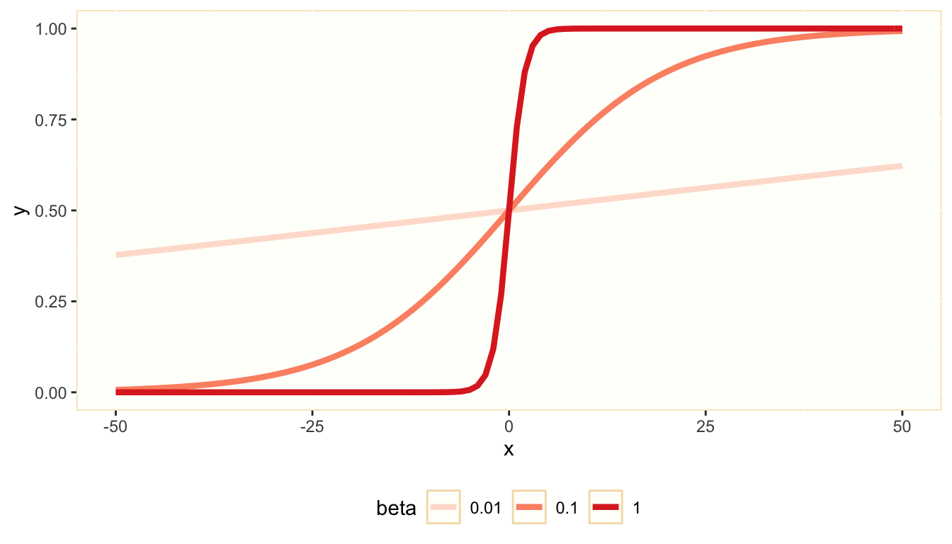
In the logit model, we use the logistic function to transform an unrestricted real variable \(z_i\) into a probability \(\pi_i\). Here is a representation of the logistic function \(y = 1/\left(1 + e^{\beta s}\right)\)
The variable \(z\) is the log odds ratio of the dependent variable being equal to one:
\[ ln\left( \frac{\pi_i}{1-\pi_i} \right) = \mathcal{\theta}' \mathcal{x}_i \]
The estimation of model coefficients is completely different from ordinary least squares. The likelihood function of the parameters given the data is a binomial distribution:
\[ \mathcal{L}\left( \mathcal{\theta} \right) = \prod_{i=1}^n \pi_i^{y_i} \left(1-\pi_i\right)^{1-y_i} \]
For simplicity, we optimize the log likelihood function to obtain the estimators:
\[ \mathcal{l}\left( \mathcal{\theta} \right) = \sum_{i=1}^n y_i\text{log} \pi_i + \sum_{i=1}^n\left(1-y_i\right) \text{log}\left(1-\pi_i\right) \]
As \(\pi_i\) is a function of dependent variables, we can obtain estimates \(b_0, \dots, b_p\) of \(\beta_0, \dots, \beta_p\) maximizing the log likelihood function \(\mathcal{l}\). Unlike ordinary least squares, there is no analytical solution for the maximization of log likelihood, so model estimates are obtained numerically.
An example of logistic regression
Let’s use the iris dataset to build a logistic regression model with a dependent variable is_virginica equal to one if the observation belongs to this species and zero otherwise. I will remove the original Species variable and Petal.Width. The later is highly correlated with the rest of predictors.
iris_logistic <- iris %>%
  mutate(is_virginica = ifelse(Species == "virginica", 1, 0)) %>%
  select(-c(Petal.Width, Species))
We can fit a logit model in R using the base function glm for generalized linear models with family = "binomial". We can use summary to obtain a summary of model output.
mod1 <- glm(is_virginica ~ ., family = "binomial", data = iris_logistic)
summary(mod1)
##
## Call:
## glm(formula = is_virginica ~ ., family = "binomial", data = iris_logistic)
##
## Deviance Residuals:
## Min 1Q Median 3Q Max
## -2.83416 -0.01085 0.00000 0.00674 1.52165
##
## Coefficients:
## Estimate Std. Error z value Pr(>|z|)
## (Intercept) -38.2154 14.0532 -2.719 0.006541 **
## Sepal.Length -3.8524 1.7091 -2.254 0.024190 *
## Sepal.Width -0.6385 2.2906 -0.279 0.780424
## Petal.Length 13.1475 3.9057 3.366 0.000762 ***
## ---
## Signif. codes: 0 '***' 0.001 '**' 0.01 '*' 0.05 '.' 0.1 ' ' 1
##
## (Dispersion parameter for binomial family taken to be 1)
##
## Null deviance: 190.954 on 149 degrees of freedom
## Residual deviance: 23.772 on 146 degrees of freedom
## AIC: 31.772
##
## Number of Fisher Scoring iterations: 10Model coefficients
Model coefficients significance allow using the logistic regression model as a explanatory tool, detecting the antecedents of the probability of each observation being virginica. We can obtain information on model coefficients in tabular form using the tidy function of the broom package.
tidy(mod1)## # A tibble: 4 x 5
## term estimate std.error statistic p.value
## <chr> <dbl> <dbl> <dbl> <dbl>
## 1 (Intercept) -38.2 14.1 -2.72 0.00654
## 2 Sepal.Length -3.85 1.71 -2.25 0.0242
## 3 Sepal.Width -0.639 2.29 -0.279 0.780
## 4 Petal.Length 13.1 3.91 3.37 0.000762The p.value column presents the probability of observing a regression coefficient equal or larger than the estimate if the null hypothesis that the regression coefficient is zero holds. We usually discard that null hypothesis for p-values equal or smaller than 0.05. Observing the sign of significant coefficients we can conclude that virginica flowers will tend to have small values of Sepal.Length and high values of Petal.Length.
We can examine the predictions for each observation using the augment function of broom. The values of the log odds \(z_i\) are found on the .fitted column, so we need to transform it to obtain the predicted probability prod.
mod1_pred <- augment(mod1) %>%
  mutate(prob = 1/(1 + exp(-.fitted)),
         is_virginica = as.factor(is_virginica))
Let’s examine the relationship between Petal.Length and prob, together with the real classification of each observation:
mod1_pred %>%
  ggplot(aes(Petal.Length, prob, color = is_virginica)) +
  geom_point() +
  theme(panel.background = element_rect(fill = "#FFFFFA", color = "#F5DEB3"), legend.key = element_rect(fill = "#FFFFFA", color = "#F5DEB3"), legend.background = element_rect(fill = "#FFFFFF", color = "#FFFFFF"), legend.position = "bottom") +
  scale_color_manual(name = "class", label = c("not virginica", "virginica"), values = c("#FF6666", "#00CC66"))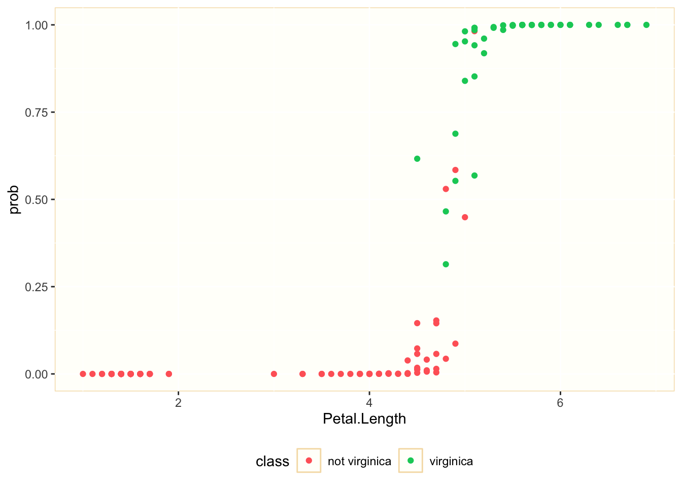
We observe that we can separate many of the observations belonging to each class considering the values of Petal.Length. Let’s see how good is Sepal.Length to explain the probability of being virginica:
mod1_pred %>%
  ggplot(aes(Sepal.Length, prob, color = is_virginica)) +
  geom_point() +
  theme(panel.background = element_rect(fill = "#FFFFFA", color = "#F5DEB3"), legend.key = element_rect(fill = "#FFFFFA", color = "#F5DEB3"), legend.background = element_rect(fill = "#FFFFFF", color = "#FFFFFF"), legend.position = "bottom") +
  scale_color_manual(name = "class", label = c("not virginica", "virginica"), values = c("#FF6666", "#00CC66"))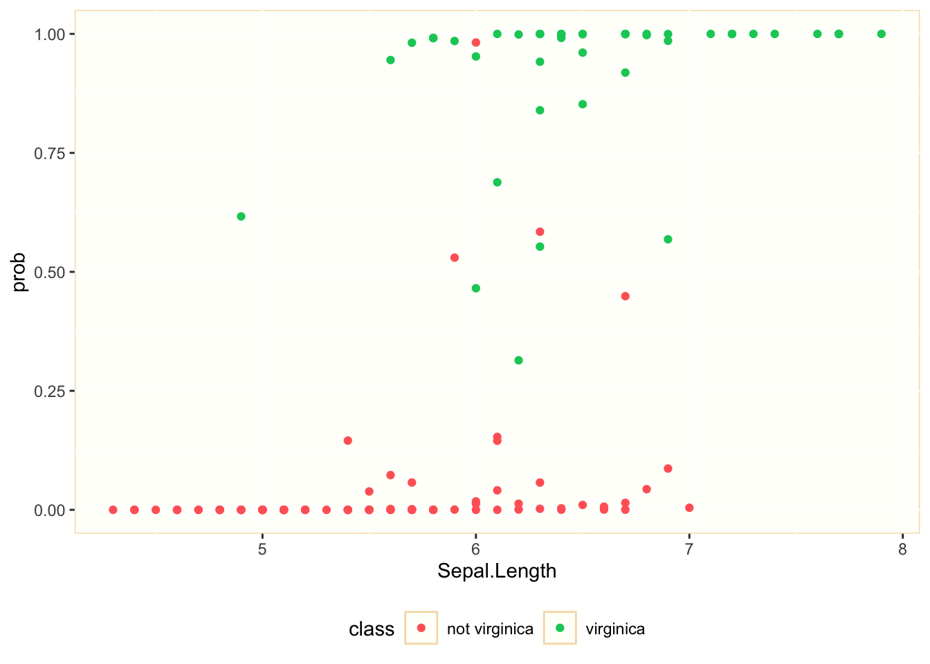
We observe that the explanatory power of Petal.Length is smaller. For values of Petal.Length between 5.5. and 7 we can find observations belonging to both classes. This was to be expected, as its p-value was much higher than Petal.Lenght, although still below 0.05.
Model fit
To assess overall significance of the model, we have only parameters related with log likelihood maximization. The F-test of overall significance and the coefficient of determination of linear regression are not available for logistic regression.
The most useful parameter to examine model fit of logistic regression is deviance. Deviance \(D\) aaccounts for how much does the model deviates from a model with perfect fit. The smaller the deviance, the better the model. Deviance is calculated as:
\[D = -2\mathcal{l}\left( \mathcal{\theta} \right)\]
The McFadden pseudo-R squared allows obtaining a fit parameter similar to linear regression’s R squared comparing the deviance of the model with the deviance of the null model \(D_{null}\). The null model does not have predictors, so it is supposed to have the worse value of fit. The formula of McFadden pseudo-R squared is:
\[R^2_{pseudo} = 1 - \frac{D}{D_{null}} = 1 - \frac{\mathcal{l}}{\mathcal{l}_{null}}\]
Note that pseudo-R squared makes sense only if log likelihood is negative.
We can obtain fit indices for our model using the glance function of broom. We can easily add the pseudo-R squared usign deviance values.
glance(mod1) %>%
  mutate(pseudo.rsq = 1 - deviance/null.deviance) %>%
  glimpse()
## Rows: 1
## Columns: 9
## $ null.deviance <dbl> 190.9543
## $ df.null <int> 149
## $ logLik <dbl> -11.8859
## $ AIC <dbl> 31.7718
## $ BIC <dbl> 43.81434
## $ deviance <dbl> 23.7718
## $ df.residual <int> 146
## $ nobs <int> 150
## $ pseudo.rsq <dbl> 0.8755105Predictions
We can use logistic regression as a predictive model for classification. We use a threshold value of probability to assign each observation to each class. Here we will assign to class virginica observations with predicted probability higher than 0.5:
pred_iris <- augment(mod1) %>%
  mutate(prob = 1/(1 + exp(-.fitted))) %>%
  mutate(pred_virginica = ifelse(prob > 0.5, 1, 0))
Once we have predicted the class, we can obtain the confusion matrix with the conf_mat function of tidymodel’s yardstick package:
library(yardstick)
pred_iris %>%
  mutate(is_virginica = as.factor(is_virginica), pred_virginica = as.factor(pred_virginica)) %>%
conf_mat(truth = is_virginica,
         estimate = pred_virginica)
## Truth
## Prediction 0 1
## 0 97 2
## 1 3 48We observe that mod1 has a good performance as classifier for this dataset.
Explaining and predicting with logistic regression
In this post, we have introduced logistic regression as a generalization of linear regression to estimate the probability of an observation being equal to one when the dependent variable is binary. Logistic regression models are estimated maximizing log likelihood.
Logistic regression can be used as a explanatory model of the antecedents of the dependent variable. This is the most common use of logistic regression in econometrics. We examine the significance of model coefficients to find antecedents of the binary dependent variable.
Another use of logistic regression is as a predictive model. When we assign a category to each observation based on predicted probability, we have a classification model. Many classification techniques of machine learning, like neural networks, can be seen as extensions of logistic regression.
References
- FAQ: What are pseudo R- squareds? https://stats.idre.ucla.edu/other/mult-pkg/faq/general/faq-what-are-pseudo-r-squareds/
Built with R 4.1.0, tidyverse 1.3.1, broom 0.7.7 and yardstick 0.0.8