When we ned to predict a continuous variable, it is frequent to use a log transformation when it is right-skewed. Here I will discuss why and how should be doing so in the context of a prediction job with the tidymodels workflow, and how can we obtain a predicted value of the original variable.
Apart from tidymodels I am using corrplot to display a correlation matrix, patchwork to present two plots together and kableExtra to present HTML tables.
library(tidymodels)
library(corrplot)
library(patchwork)
library(kableExtra)
I will use the diamonds dataset included with ggplot2, that contains the prices and other attributes of almost 54,000 diamonds:
diamonds %>% glimpse()## Rows: 53,940
## Columns: 10
## $ carat <dbl> 0.23, 0.21, 0.23, 0.29, 0.31, 0.24, 0.24, 0.26, 0.22, 0.23, 0.…
## $ cut <ord> Ideal, Premium, Good, Premium, Good, Very Good, Very Good, Ver…
## $ color <ord> E, E, E, I, J, J, I, H, E, H, J, J, F, J, E, E, I, J, J, J, I,…
## $ clarity <ord> SI2, SI1, VS1, VS2, SI2, VVS2, VVS1, SI1, VS2, VS1, SI1, VS1, …
## $ depth <dbl> 61.5, 59.8, 56.9, 62.4, 63.3, 62.8, 62.3, 61.9, 65.1, 59.4, 64…
## $ table <dbl> 55, 61, 65, 58, 58, 57, 57, 55, 61, 61, 55, 56, 61, 54, 62, 58…
## $ price <int> 326, 326, 327, 334, 335, 336, 336, 337, 337, 338, 339, 340, 34…
## $ x <dbl> 3.95, 3.89, 4.05, 4.20, 4.34, 3.94, 3.95, 4.07, 3.87, 4.00, 4.…
## $ y <dbl> 3.98, 3.84, 4.07, 4.23, 4.35, 3.96, 3.98, 4.11, 3.78, 4.05, 4.…
## $ z <dbl> 2.43, 2.31, 2.31, 2.63, 2.75, 2.48, 2.47, 2.53, 2.49, 2.39, 2.…Our job will be predicting the price of diamonds from their attributes.
Exploratory analysis
Let’s start examining the correlations between numerical variables.
cor_diamonds <- diamonds %>%
  select(where(is.numeric)) %>%
  cor()
Let’s use corrplot to examine the correlations:
corrplot.mixed(cor_diamonds, order = "hclust")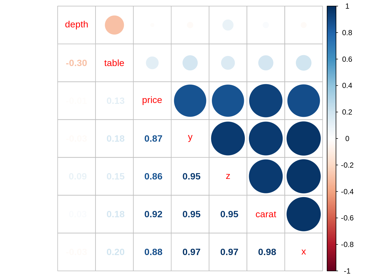
We observe that carat, x, y and z are highly correlated with price and among themselves. In line with other analysis, I have kept carat and discarded x, y and z.
Let’s go now to the distribution of price:
ggplot(diamonds, aes(price)) +
  geom_histogram(bins = 30) +
  theme_minimal() +
  labs(title = "Distribution of price")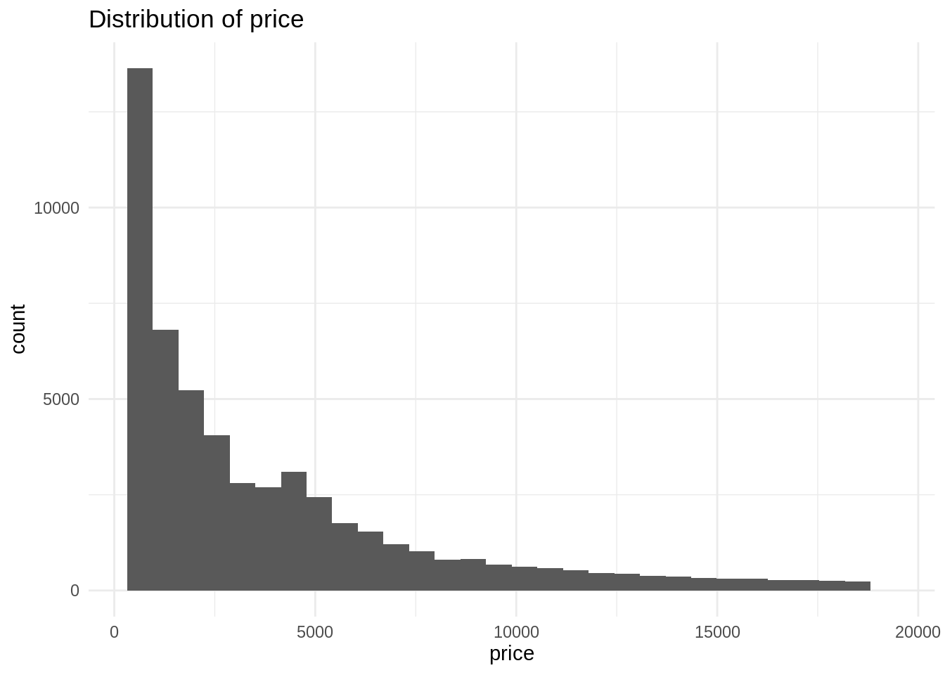
The histogram shows that price is a right skewed distribution, as has a long tail in the right hand side of the distribution. This means that some diamonds have a very large price, compared with the whole of the distribution. Something similar happens usually with variables housing price, income and other variables relevant in economics.
Let’s examine the distribution of the decimal logarithm of price.
ggplot(diamonds, aes(price)) +
  geom_histogram(bins = 30) +
  theme_minimal() +
  scale_x_log10() +
  labs(title = "Distribution of logarithm of price")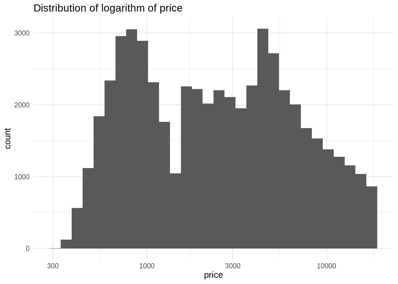
We observe a bimodal normal distribution. In general, the log of a right-skewed distribution looks similar to a normal distribution. This means that we will obtain better estimators in a regression model using the log transformation, as the residuals of the model will tend to be normal.
Let’s add a log_price variable to the dataset, that we will be using later in the prediction job.
diamonds <- diamonds %>%
  mutate(log_price = log10(price))
To end with the exploratory data analysis section, let’s examine the relationship between carat and log_price.
ggplot(diamonds, aes(carat, price)) +
  geom_point() +
  geom_smooth() +
  scale_x_log10() +
  theme_minimal() +
  labs(title = "Relationship between carat and price")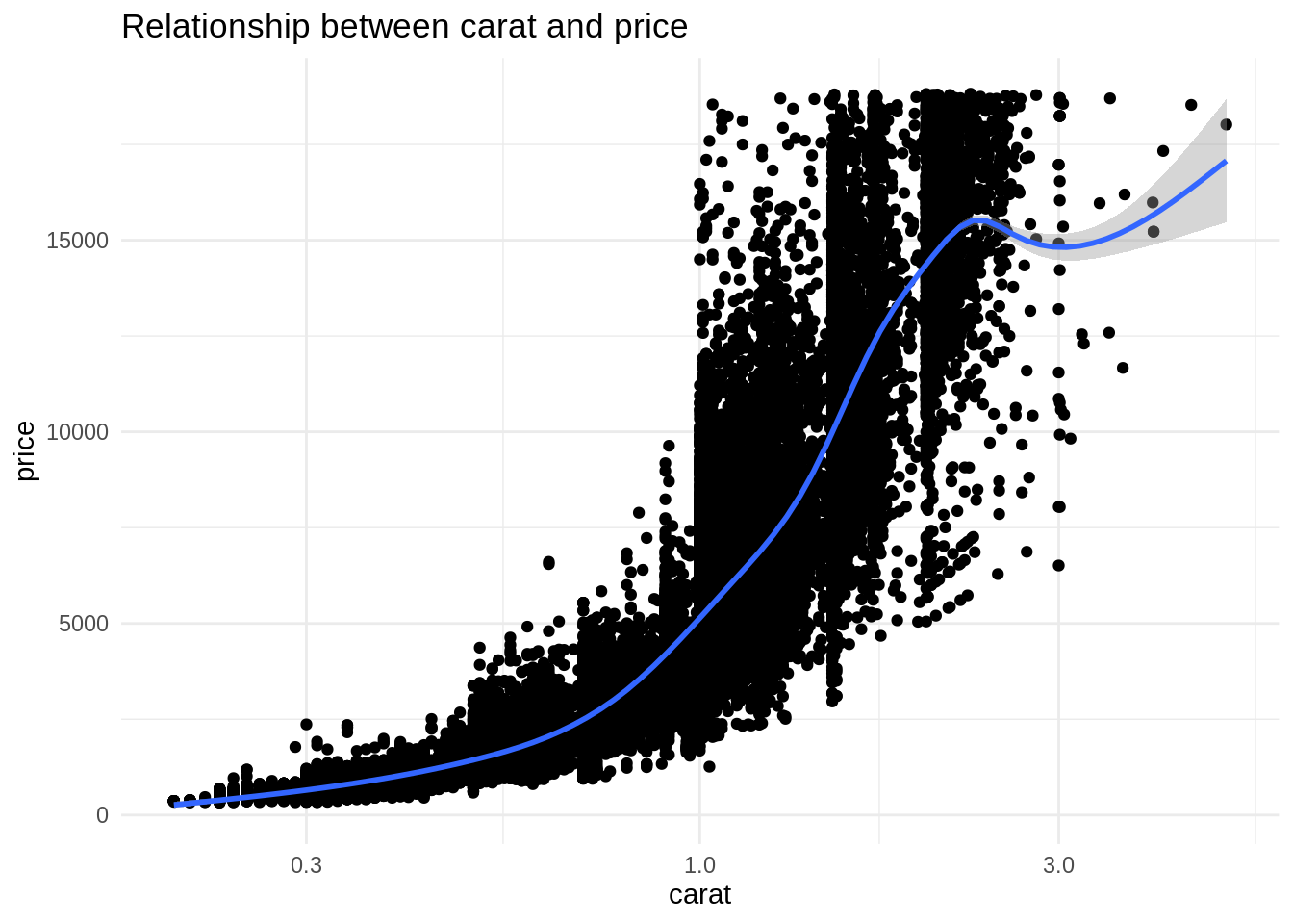
This relationship is nonlinear, so the model could benefit of the addition of a quadratic term.
Predicting the price
To check the opportunity of using the log variable, I will predict using the original price variable. The workflow starts by splitting the data into train and test sets, stratifying by the target variable. I am doing this to get a similar distribution of price in the train and test sets.
set.seed(1111)
split_price <- initial_split(diamonds, prop = 0.9, strata = price)
The rec_price recipe includes the transformations for this model:
- removing variables with
step_rm. - adding a quadratic term to carat with
step_poly. - transforming categorical variables to a set of dummies generated with one hot encoding with
step_dummy. - removing near zero variance variables with
step_nzv.
rec_price <- training(split_price) %>%
  recipe(price ~ .) %>%
  step_rm(log_price, x, y, z) %>%
  step_poly(carat, degree = 2) %>%
  step_dummy(all_nominal(), one_hot = TRUE) %>%
  step_nzv(all_predictors()) %>%
  step_rm(color_1)
Here is the result of the recipe:
rec_price %>% prep() %>% juice() %>% glimpse()## Rows: 48,545
## Columns: 21
## $ depth <dbl> 59.8, 56.9, 62.4, 63.3, 62.8, 62.3, 61.9, 65.1, 59.4, 64.…
## $ table <dbl> 61, 65, 58, 58, 57, 57, 55, 61, 61, 55, 56, 61, 54, 62, 5…
## $ price <int> 326, 327, 334, 335, 336, 336, 337, 337, 338, 339, 340, 34…
## $ carat_poly_1 <dbl> -0.005631217, -0.005439625, -0.004864846, -0.004673253, -…
## $ carat_poly_2 <dbl> 0.006116938, 0.005640942, 0.004280652, 0.003849787, 0.005…
## $ cut_2 <dbl> 0, 1, 0, 1, 0, 0, 0, 0, 0, 1, 0, 0, 0, 0, 0, 0, 1, 0, 1, …
## $ cut_3 <dbl> 0, 0, 0, 0, 1, 1, 1, 0, 1, 0, 0, 0, 0, 0, 0, 0, 0, 1, 0, …
## $ cut_4 <dbl> 1, 0, 1, 0, 0, 0, 0, 0, 0, 0, 0, 1, 0, 1, 1, 0, 0, 0, 0, …
## $ cut_5 <dbl> 0, 0, 0, 0, 0, 0, 0, 0, 0, 0, 1, 0, 1, 0, 0, 1, 0, 0, 0, …
## $ color_2 <dbl> 1, 1, 0, 0, 0, 0, 0, 1, 0, 0, 0, 0, 0, 1, 1, 0, 0, 0, 0, …
## $ color_3 <dbl> 0, 0, 0, 0, 0, 0, 0, 0, 0, 0, 0, 1, 0, 0, 0, 0, 0, 0, 0, …
## $ color_4 <dbl> 0, 0, 0, 0, 0, 0, 0, 0, 0, 0, 0, 0, 0, 0, 0, 0, 0, 0, 0, …
## $ color_5 <dbl> 0, 0, 0, 0, 0, 0, 1, 0, 1, 0, 0, 0, 0, 0, 0, 0, 0, 0, 0, …
## $ color_6 <dbl> 0, 0, 1, 0, 0, 1, 0, 0, 0, 0, 0, 0, 0, 0, 0, 1, 0, 0, 1, …
## $ color_7 <dbl> 0, 0, 0, 1, 1, 0, 0, 0, 0, 1, 1, 0, 1, 0, 0, 0, 1, 1, 0, …
## $ clarity_2 <dbl> 0, 0, 0, 1, 0, 0, 0, 0, 0, 0, 0, 0, 1, 1, 0, 1, 0, 0, 1, …
## $ clarity_3 <dbl> 1, 0, 0, 0, 0, 0, 1, 0, 0, 1, 0, 1, 0, 0, 0, 0, 1, 1, 0, …
## $ clarity_4 <dbl> 0, 0, 1, 0, 0, 0, 0, 1, 0, 0, 0, 0, 0, 0, 0, 0, 0, 0, 0, …
## $ clarity_5 <dbl> 0, 1, 0, 0, 0, 0, 0, 0, 1, 0, 1, 0, 0, 0, 0, 0, 0, 0, 0, …
## $ clarity_6 <dbl> 0, 0, 0, 0, 1, 0, 0, 0, 0, 0, 0, 0, 0, 0, 0, 0, 0, 0, 0, …
## $ clarity_7 <dbl> 0, 0, 0, 0, 0, 1, 0, 0, 0, 0, 0, 0, 0, 0, 0, 0, 0, 0, 0, …Let’s define a straightforward linear model…
lm <- linear_reg(mode = "regression") %>%
  set_engine("lm")
… and fit the model and the recipe with a workflow:
model_price <- workflow() %>%
  add_recipe(rec_price) %>%
  add_model(lm) %>%
  fit(training(split_price))
We obtain the predicted values of price with pred_price…
pred_price <- model_price %>%
  predict(training(split_price)) %>%
  bind_cols(training(split_price))
… And here it is the real versus predicted variables plot:
ggplot(pred_price, aes(price, .pred)) +
  geom_point() +
  geom_abline(slope = 1, intercept = 0, color = "red") +
  theme_minimal() +
  labs(title = "Real versus predicted values (price model)", x = "price", y = "pred. price")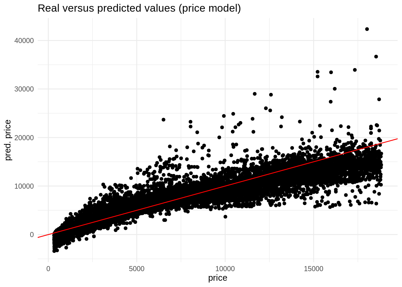
The result of this model is problematic, as it return negative prices for some observations. We can also avoid that with a log transformation. The logarithm can take any value, but it is only defined for positive values.
Finally, let’s define the metrics we will be using in this job:
metric_prediction <- metric_set(rsq, mae, rmse)The values of the metrics in the train test of this model are:
metrics_price <- pred_price %>%
  metric_prediction(truth = price, estimate = .pred) %>%
  mutate(.model = "price") %>%
  select(-.estimator)

metrics_price
## # A tibble: 3 × 3
## .metric .estimate .model
## <chr> <dbl> <chr>
## 1 rsq 0.899 price
## 2 mae 814. price
## 3 rmse 1264. pricePredicting with log
Let’s do the same job, but predicting the log of the target variable log_price. Let’s start with a new split, now with log_price as the stratifying variable.
set.seed(1111)
split_log <- initial_split(diamonds, prop = 0.9, strata = log_price)
The recipe is quite similar to the previous model:
rec_log <- training(split_log) %>%
  recipe(log_price ~ .) %>%
  step_rm(price, x, y, z) %>%
  step_poly(carat, degree = 2) %>%
  step_dummy(all_nominal(), one_hot = TRUE) %>%
  step_nzv(all_predictors()) %>%
  step_rm(color_1)
I am fitting the same lm model, but with the rec_log recipe:
model_log <- workflow() %>%
  add_recipe(rec_log) %>%
  add_model(lm) %>%
  fit(training(split_log))
And then we can predict the train set. Note that we will obtain a prediction of the log of price in the .pred column.
pred_log <- model_log %>%
  predict(training(split_log)) %>%
  bind_cols(training(split_log))
If we want a predicted value of price, we need to undo the log transformation in the predicted variable. We do that in .pred_price.
pred_log <- pred_log %>%
  mutate(.pred_price = 10^.pred)
Here is the result of plotting the real and predicted variables in the train set for price and its log. We observe now that we do not have negative values of price.
log <- ggplot(pred_log, aes(log_price, .pred)) +
  geom_point() +
  geom_abline(slope = 1, intercept = 0, color = "red") +
  theme_minimal() +
  labs(title = "Log real versus log predicted (log model)", x = "price (log)", y = "pred. price (log)")

real <- ggplot(pred_log, aes(price, .pred_price)) +
  geom_point() +
  geom_abline(slope = 1, intercept = 0, color = "red") +
  theme_minimal() +
  labs(title = "Real versus predicted (log model)", x = "price", y = "pred. price")

log + real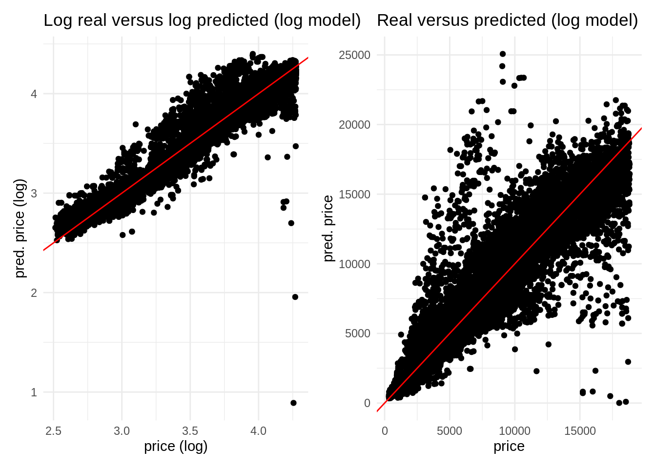
Let’s examine the metrics for the log of price:
metrics_log <- pred_log %>%
  metric_prediction(truth = log_price, estimate = .pred) %>%
  mutate(.model = "log") %>%
  select(-.estimator)

metrics_log
## # A tibble: 3 × 3
## .metric .estimate .model
## <chr> <dbl> <chr>
## 1 rsq 0.965 log
## 2 mae 0.0582 log
## 3 rmse 0.0822 logAnd then with price itself.
metrics_log_price <- pred_log %>%
  metric_prediction(truth = price, estimate = .pred_price) %>%
  mutate(.model = "price with log") %>%
  select(-.estimator)

metrics_log_price
## # A tibble: 3 × 3
## .metric .estimate .model
## <chr> <dbl> <chr>
## 1 rsq 0.924 price with log
## 2 mae 528. price with log
## 3 rmse 1123. price with logComparing metrics
Let’s compare how well performs each model putting side to side the metrics of both models. We can do that because tidymodels offers us the metrics as data frames that can be put together easily.
bind_rows(metrics_price, metrics_log_price) %>%
  mutate(.estimate = format(.estimate, digits = 3)) %>%
  pivot_wider(id_cols = ".metric", names_from = ".model", values_from = ".estimate") %>%
  kbl(align = c("l", "r", "r")) %>%
kable_styling(bootstrap_options = c("striped", "condensed", "responsive", "hover"), full_width = FALSE)| .metric | price | price with log |
|---|---|---|
| rsq | 0.899 | 0.924 |
| mae | 813.541 | 528.007 |
| rmse | 1263.751 | 1123.007 |
For the training test, the log model performs better than the price model. Let’s see how well each model performs in the test set.
pred_price_test <- model_price %>%
  predict(testing(split_price)) %>%
  bind_cols(testing(split_price))

pred_log_test <- model_log %>%
  predict(testing(split_log)) %>%
  bind_cols(testing(split_log)) %>%
  mutate(.pred_price = 10^.pred)

metrics_price_test <- pred_price_test %>%
  metric_prediction(truth = price, estimate = .pred) %>%
  mutate(.model = "price") %>%
  select(-.estimator)

metrics_log_test <- pred_log_test %>%
  metric_prediction(truth = price, estimate = .pred_price) %>%
  mutate(.model = "price with log") %>%
  select(-.estimator)

bind_rows(metrics_price_test, metrics_log_test) %>%
  mutate(.estimate = format(.estimate, digits = 3)) %>%
  pivot_wider(id_cols = ".metric", names_from = ".model", values_from = ".estimate") %>%
  kbl(align = c("l", "r", "r")) %>%
kable_styling(bootstrap_options = c("striped", "condensed", "responsive", "hover"), full_width = FALSE)| .metric | price | price with log |
|---|---|---|
| rsq | 0.908 | 0.923 |
| mae | 811.561 | 537.652 |
| rmse | 1226.000 | 1167.739 |
Again, the log transformation has better performance in the test set.
References
- Cross validated. What is the reason the log transformation is used with right-skewed distributions? https://stats.stackexchange.com/questions/107610/what-is-the-reason-the-log-transformation-is-used-with-right-skewed-distribution
- Wei, Taiyun; Simko, Viliam (2021). An Introduction to corrplot Package. https://cran.r-project.org/web/packages/corrplot/vignettes/corrplot-intro.html
Session info
## R version 4.2.0 (2022-04-22)
## Platform: x86_64-pc-linux-gnu (64-bit)
## Running under: Linux Mint 19.2
##
## Matrix products: default
## BLAS:   /usr/lib/x86_64-linux-gnu/openblas/libblas.so.3
## LAPACK: /usr/lib/x86_64-linux-gnu/libopenblasp-r0.2.20.so
##
## locale:
##  [1] LC_CTYPE=es_ES.UTF-8       LC_NUMERIC=C
##  [3] LC_TIME=es_ES.UTF-8        LC_COLLATE=es_ES.UTF-8
##  [5] LC_MONETARY=es_ES.UTF-8    LC_MESSAGES=es_ES.UTF-8
##  [7] LC_PAPER=es_ES.UTF-8       LC_NAME=C
##  [9] LC_ADDRESS=C               LC_TELEPHONE=C
## [11] LC_MEASUREMENT=es_ES.UTF-8 LC_IDENTIFICATION=C
##
## attached base packages:
## [1] stats     graphics  grDevices utils     datasets  methods   base
##
## other attached packages:
##  [1] kableExtra_1.3.4   patchwork_1.1.1    corrplot_0.92      yardstick_0.0.9
##  [5] workflowsets_0.2.1 workflows_0.2.6    tune_0.2.0         tidyr_1.2.0
##  [9] tibble_3.1.6       rsample_0.1.1      recipes_0.2.0      purrr_0.3.4
## [13] parsnip_0.2.1      modeldata_0.1.1    infer_1.0.0        ggplot2_3.3.5
## [17] dplyr_1.0.9        dials_0.1.1        scales_1.2.0       broom_0.8.0
## [21] tidymodels_0.2.0
##
## loaded via a namespace (and not attached):
##  [1] nlme_3.1-157       lubridate_1.8.0    webshot_0.5.3      httr_1.4.2
##  [5] DiceDesign_1.9     tools_4.2.0        backports_1.4.1    bslib_0.3.1
##  [9] utf8_1.2.2         R6_2.5.1           rpart_4.1.16       mgcv_1.8-40
## [13] DBI_1.1.2          colorspace_2.0-3   nnet_7.3-17        withr_2.5.0
## [17] tidyselect_1.1.2   compiler_4.2.0     rvest_1.0.2        cli_3.3.0
## [21] xml2_1.3.3         labeling_0.4.2     bookdown_0.26      sass_0.4.1
## [25] systemfonts_1.0.4  stringr_1.4.0      digest_0.6.29      svglite_2.1.0
## [29] rmarkdown_2.14     pkgconfig_2.0.3    htmltools_0.5.2    parallelly_1.31.1
## [33] lhs_1.1.5          highr_0.9          fastmap_1.1.0      rlang_1.0.2
## [37] rstudioapi_0.13    farver_2.1.0       jquerylib_0.1.4    generics_0.1.2
## [41] jsonlite_1.8.0     magrittr_2.0.3     Matrix_1.4-1       Rcpp_1.0.8.3
## [45] munsell_0.5.0      fansi_1.0.3        GPfit_1.0-8        lifecycle_1.0.1
## [49] furrr_0.3.0        stringi_1.7.6      pROC_1.18.0        yaml_2.3.5
## [53] MASS_7.3-57        plyr_1.8.7         grid_4.2.0         parallel_4.2.0
## [57] listenv_0.8.0      crayon_1.5.1       lattice_0.20-45    splines_4.2.0
## [61] knitr_1.39         pillar_1.7.0       future.apply_1.9.0 codetools_0.2-18
## [65] glue_1.6.2         evaluate_0.15      blogdown_1.9       vctrs_0.4.1
## [69] foreach_1.5.2      gtable_0.3.0       future_1.25.0      assertthat_0.2.1
## [73] xfun_0.30          gower_1.0.0        prodlim_2019.11.13 viridisLite_0.4.0
## [77] class_7.3-20       survival_3.2-13    timeDate_3043.102  iterators_1.0.14
## [81] hardhat_0.2.0      lava_1.6.10        globals_0.14.0     ellipsis_0.3.2
## [85] ipred_0.9-12