Linear regression si about finding a linear relationship between:
- a dependent variable, also called endogenous, response or criterion \(y\)
- and a set \(p\) of independent variables, sometimes called exogenous or predictor \(x_j\).
The posited relationship can be represented as:
\[ y_i = \beta_0 + \beta_1x_{i1} + \dots + \beta_px_{ip} + \varepsilon_i \]
Linear regression is one of the more powerful tools of statistical data analysis. In its many variants, we use linear regression:
- to explain relationships between dependent and independent variables, trying to find if we can assert that regression coefficients \(\beta_j\) are significantly different from zero.
- to predict the dependent variable, in the context of supervised learning.
The above equations are defined for the whole population. We usually have a sample, from which we can make statistical inferences about the regression coefficients. We will never know \(\beta_j\), but its estimator \(b_j\):
\[ y_i = b_0 + b_1x_{i1} + \dots + b_px_{ip} + e_i \]
From these estimators, we can find predictors \(\hat{y}_i\) for each observation, as an alternative of estimating all observations through the mean \(\bar{y}\):
\[ \hat{y}_i = b_0 + b_1x_{i1} + \dots + b_px_{ip} + e_i \]
\[ y_i = \hat{y}_i + e_i \]
The most common way of obtaining the estimators \(b_j\) is through ordinary least squares (OLS). These are the estimators that minimize:
\[ \sum e_i^2 \]
Linear regression on mtcars
R has a built-in function lm that calculates the OLS estimators for a set of dependent and independent variables. We don’t need any package for lm, but we will use some packages:
- the
tidyversefor data handling and plotting, broomto tidy the output of lm- and
ggfortifyto present some plots for the linear model.
library(tidyverse)
library(broom)
library(ggfortify)
I will examine the mtcars dataset, to find an explanatory model of fuel consumption mpg.
mtcars %>% glimpse()## Rows: 32
## Columns: 11
## $ mpg <dbl> 21.0, 21.0, 22.8, 21.4, 18.7, 18.1, 14.3, 24.4, 22.8, 19.2, 17.8,…
## $ cyl <dbl> 6, 6, 4, 6, 8, 6, 8, 4, 4, 6, 6, 8, 8, 8, 8, 8, 8, 4, 4, 4, 4, 8,…
## $ disp <dbl> 160.0, 160.0, 108.0, 258.0, 360.0, 225.0, 360.0, 146.7, 140.8, 16…
## $ hp <dbl> 110, 110, 93, 110, 175, 105, 245, 62, 95, 123, 123, 180, 180, 180…
## $ drat <dbl> 3.90, 3.90, 3.85, 3.08, 3.15, 2.76, 3.21, 3.69, 3.92, 3.92, 3.92,…
## $ wt <dbl> 2.620, 2.875, 2.320, 3.215, 3.440, 3.460, 3.570, 3.190, 3.150, 3.…
## $ qsec <dbl> 16.46, 17.02, 18.61, 19.44, 17.02, 20.22, 15.84, 20.00, 22.90, 18…
## $ vs <dbl> 0, 0, 1, 1, 0, 1, 0, 1, 1, 1, 1, 0, 0, 0, 0, 0, 0, 1, 1, 1, 1, 0,…
## $ am <dbl> 1, 1, 1, 0, 0, 0, 0, 0, 0, 0, 0, 0, 0, 0, 0, 0, 0, 1, 1, 1, 0, 0,…
## $ gear <dbl> 4, 4, 4, 3, 3, 3, 3, 4, 4, 4, 4, 3, 3, 3, 3, 3, 3, 4, 4, 4, 3, 3,…
## $ carb <dbl> 4, 4, 1, 1, 2, 1, 4, 2, 2, 4, 4, 3, 3, 3, 4, 4, 4, 1, 2, 1, 1, 2,…I will transform variables from vs to carb to factors, as they are categoric rather than numeric:
mtcars <- mtcars %>%
  mutate_at(vars(vs:carb), as.factor)
A regression model
Let’s examine a linear regression model that includes all the possible independent variables. The inputs of lm are:
- a formula
mpg ~ .meaning thatmpgis the dependent variable and the rest of variables of the dataset are the independent variables. - a data frame
mtcarswith data to build the model. Formula variables must match column names of the data frame.
Unlike other statistical software like Stata or SPSS, we store the result of estimating the model into a variable mod0.
mod0 <- lm(mpg ~ ., mtcars)The standard way of presenting the results of a linear model is through summary:
summary(mod0)##
## Call:
## lm(formula = mpg ~ ., data = mtcars)
##
## Residuals:
## Min 1Q Median 3Q Max
## -3.6533 -1.3325 -0.5166 0.7643 4.7284
##
## Coefficients:
## Estimate Std. Error t value Pr(>|t|)
## (Intercept) 25.31994 23.88164 1.060 0.3048
## cyl -1.02343 1.48131 -0.691 0.4995
## disp 0.04377 0.03058 1.431 0.1716
## hp -0.04881 0.03189 -1.531 0.1454
## drat 1.82084 2.38101 0.765 0.4556
## wt -4.63540 2.52737 -1.834 0.0853 .
## qsec 0.26967 0.92631 0.291 0.7747
## vs1 1.04908 2.70495 0.388 0.7032
## am1 0.96265 3.19138 0.302 0.7668
## gear4 1.75360 3.72534 0.471 0.6442
## gear5 1.87899 3.65935 0.513 0.6146
## carb2 -0.93427 2.30934 -0.405 0.6912
## carb3 3.42169 4.25513 0.804 0.4331
## carb4 -0.99364 3.84683 -0.258 0.7995
## carb6 1.94389 5.76983 0.337 0.7406
## carb8 4.36998 7.75434 0.564 0.5809
## ---
## Signif. codes: 0 '***' 0.001 '**' 0.01 '*' 0.05 '.' 0.1 ' ' 1
##
## Residual standard error: 2.823 on 16 degrees of freedom
## Multiple R-squared: 0.8867, Adjusted R-squared: 0.7806
## F-statistic: 8.352 on 15 and 16 DF, p-value: 6.044e-05The summary includes:
- The function call.
- A summary of the residuals \(e_i\).
- The estimators of coefficients, and the p-value of the null hypothesis that each regression coefficient is zero. In this case all p-values are above 0.05, therefore we don’t know if any of the coefficients is different from zero.
- Some parameters of overall significance of the model: the coefficient of determination (raw and adjusted), and a F-test indicating if the regression model explains the dependent variable better than the mean. Values of the adjusted coefficient of determination close to one and small values of p-value suggest good fit.
In this case we observe that the model is significant (if we take the usual convention that the p-value should be below 0.05), but that none of the coefficients is. This may arise because lack of statistical power (mtcars is a small dataset) or because of correlation among dependent variables.
The broom package offers an alternative way of presenting the output of statistical analysis. The package works through three functions:
tidypresents parameter estimators,glanceoverall model significance estimators,- and
augmentadds information to the dataset.
The output of these functions is a tibble, with a content depending of the examined model. Let’s see the outcome of tidy and glance for this model:
tidy(mod0)## # A tibble: 16 x 5
## term estimate std.error statistic p.value
## <chr> <dbl> <dbl> <dbl> <dbl>
## 1 (Intercept) 25.3 23.9 1.06 0.305
## 2 cyl -1.02 1.48 -0.691 0.500
## 3 disp 0.0438 0.0306 1.43 0.172
## 4 hp -0.0488 0.0319 -1.53 0.145
## 5 drat 1.82 2.38 0.765 0.456
## 6 wt -4.64 2.53 -1.83 0.0853
## 7 qsec 0.270 0.926 0.291 0.775
## 8 vs1 1.05 2.70 0.388 0.703
## 9 am1 0.963 3.19 0.302 0.767
## 10 gear4 1.75 3.73 0.471 0.644
## 11 gear5 1.88 3.66 0.513 0.615
## 12 carb2 -0.934 2.31 -0.405 0.691
## 13 carb3 3.42 4.26 0.804 0.433
## 14 carb4 -0.994 3.85 -0.258 0.799
## 15 carb6 1.94 5.77 0.337 0.741
## 16 carb8 4.37 7.75 0.564 0.581glance(mod0) %>% glimpse()## Rows: 1
## Columns: 12
## $ r.squared <dbl> 0.886746
## $ adj.r.squared <dbl> 0.7805703
## $ sigma <dbl> 2.823223
## $ statistic <dbl> 8.351689
## $ p.value <dbl> 6.044113e-05
## $ df <dbl> 15
## $ logLik <dbl> -67.52781
## $ AIC <dbl> 169.0556
## $ BIC <dbl> 193.9731
## $ deviance <dbl> 127.5294
## $ df.residual <int> 16
## $ nobs <int> 32A simpler regression model
Let’s try a explanatory model of fuel consumption mpg considering car weight wt only:
mod1 <- lm(mpg ~ wt, mtcars)We see that the regression coefficients of the intercept and wt are significant in this model:
tidy(mod1)## # A tibble: 2 x 5
## term estimate std.error statistic p.value
## <chr> <dbl> <dbl> <dbl> <dbl>
## 1 (Intercept) 37.3 1.88 19.9 8.24e-19
## 2 wt -5.34 0.559 -9.56 1.29e-10and that the overall significance of the model is higher than mod0:
glance(mod1) %>% select(r.squared, adj.r.squared, p.value)## # A tibble: 1 x 3
## r.squared adj.r.squared p.value
## <dbl> <dbl> <dbl>
## 1 0.753 0.745 1.29e-10Graphical diagnostics
This new, simpler model looks convincing: we expect higher fuel consumption for weighter vehicles. But to confirm that the model is adequate, we need to do residual diagnostics to confirm that:
- Residuals have mean zero and constant variance across predicted values \(\hat{y}_i\). We check that with a residuals vs fitted values plot.
- Residuals are distributed normally. We check that with a QQ-plot.
We can obtain these plots in R base doing plot(mod1, which = 1) and plot(mod2, which = 2). But we can obtain prettier versions of them with the autoplot function of ggfortify:
autoplot(mod1, which = 2:1, ncol = 2, label.size = 3)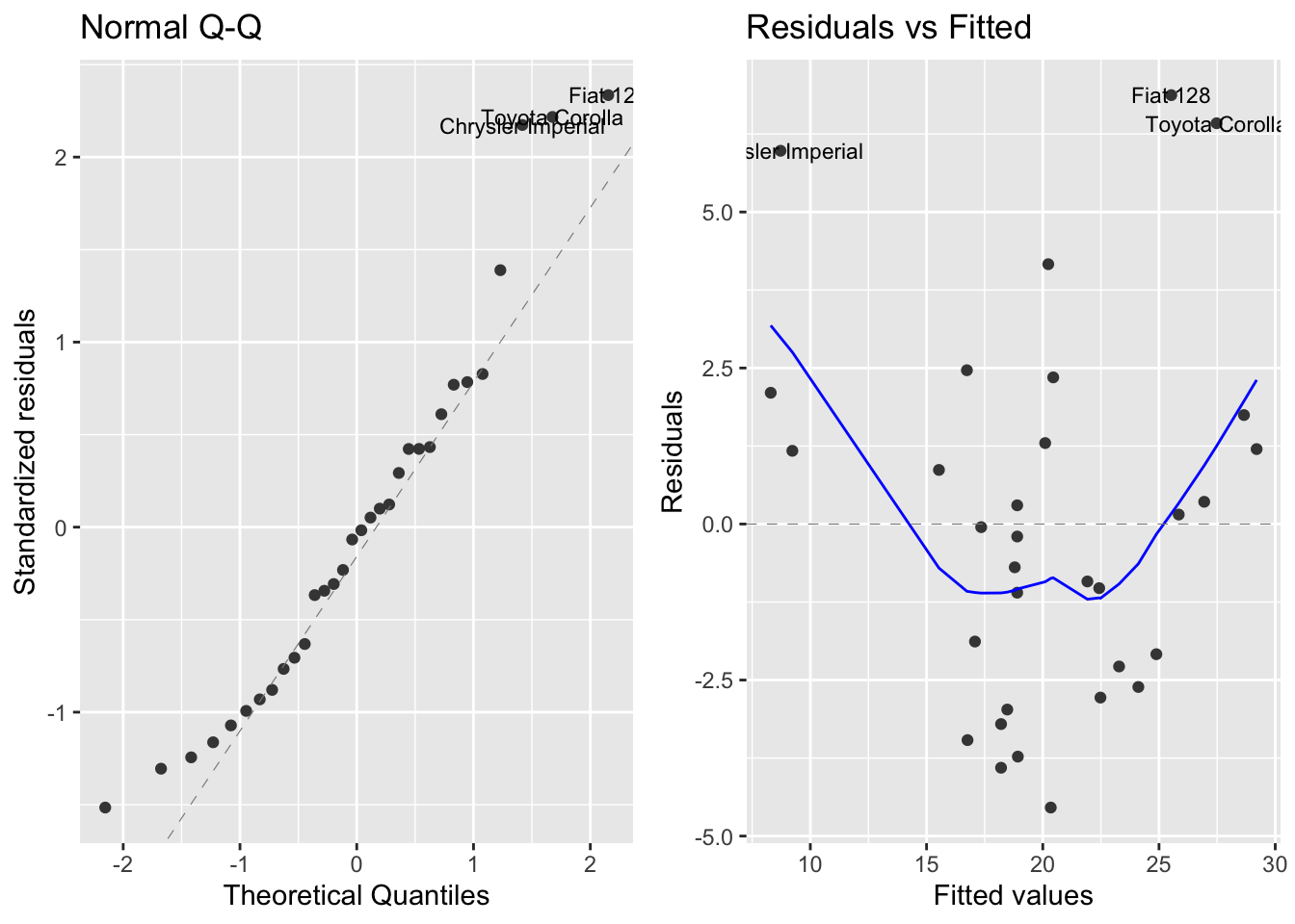
In the first plot we observe that residuals are reasonably normal. From the second plot we learn that the mean of residuals is larger for extreme values of \(\hat{y}_i\) than for central values. This suggests that the relationship between weight and fuel consumption is not linear. Let’s examine that with an alternative model.
A quadratic model
We can examine nonlinear relationships with linear regressions adding powered values of independent variables. As these powers tend to be correlated with the original value, it is better to use orthogonal polynomials (orthogonal means non-correlated) using the poly function.
mod2 <- lm(mpg ~ poly(wt, 2), mtcars)Let’s examine the regression coefficients:
tidy(mod2)## # A tibble: 3 x 5
## term estimate std.error statistic p.value
## <chr> <dbl> <dbl> <dbl> <dbl>
## 1 (Intercept) 20.1 0.469 42.9 8.75e-28
## 2 poly(wt, 2)1 -29.1 2.65 -11.0 7.52e-12
## 3 poly(wt, 2)2 8.64 2.65 3.26 2.86e- 3We observe that the regression coefficients of the first- and second-order terms are significantly different from zero. Let’s examine the residual diagnostics again:
autoplot(mod2, which = 1:2, ncol = 2, label.size = 3)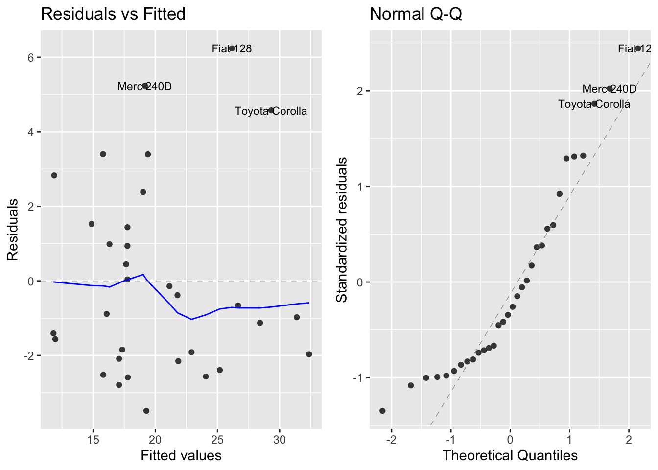
Now we see that now the residuals behave more smoothly, although we observe some outliers in the first plot. We take advantage that glance returns us a tibble to together the overall signficance metrics of the three models:
bind_rows(glance(mod0) %>% mutate(model = "all vars"),
          glance(mod1) %>% mutate(model = "wt"),
          glance(mod2) %>% mutate(model = "wt squared")) %>%
  select(model, r.squared, adj.r.squared, p.value)
## # A tibble: 3 x 4
## model r.squared adj.r.squared p.value
## <chr> <dbl> <dbl> <dbl>
## 1 all vars 0.887 0.781 6.04e- 5
## 2 wt 0.753 0.745 1.29e-10
## 3 wt squared 0.819 0.807 1.71e-11The adjusted coefficient of determination increases as we build more accurate linear regression models. So we can conclude that mod2 is the best explanatory model of mpg among the ones we have tested.
Built with R 4.0.3, tidyverse 1.3.0, broom 0.7.5 and ggoftify 0.4.11