Latin Hypercube Sampling

Jose M Sallan 2024-11-01 8 min read

Latin Hypercube Sampling (LHS) is a statistical method for generating a sample of plausible values from a multidimensional distribution. It is a type of stratified sampling, particularly useful in computer simulations and statistical experiments where multiple variables are involved. The main goal of LHS is to ensure that each parameter is sampled according to the probability distribution.

Here’s a step-by-step breakdown of how it works:

Divide the Range: Each parameter’s range is divided into equal intervals (strata). For example, if you want 10 samples, each parameter’s range is divided into 10 equal parts.
Stratify Sampling: Within each interval of every parameter, a single sample point is randomly selected. This ensures that each parameter is sampled across its entire range without redundancy.
Combine Parameter Values: The sampled values of each parameter are then randomly paired to form unique combinations, or samples, across the multidimensional space. When two variables are samples, each row and column of the grid has a single observation, thus forming a Latin square. The extrapolation of this idea to more dimensions is the Latin hypercube.

LHS is advantageous because it improves sampling efficiency. It is particularly useful in methods like Monte Carlo, when we need to simulate variables following a probability distribution.

In this post, I will introduce the lhs package to generate basic Latin hypercube samples and designs. I also use the mc2d package to model the Pert distribution, and the tidyverse and GGally for data handling and plotting.

library(tidyverse)
library(lhs)
library(GGally)
library(mc2d)

We need methods like LHS because simulating with straigth random sampling can give sets of values that do not represent the distribution adequately. To illustrate, let’s see the output of generating one thousand values of an uniform distribution.

set.seed(111)
unif_sample <- tibble(obs = runif(1000))

unif_sample |>
  ggplot(aes(obs)) +
  geom_histogram(aes(y = after_stat(count / sum(count))), fill = "#A0A0A0") +
  geom_hline(yintercept = 1/30, color = "red") +
  labs(title = "Uniform distribution (random sampling)", x = NULL, y = NULL) +
  theme_minimal()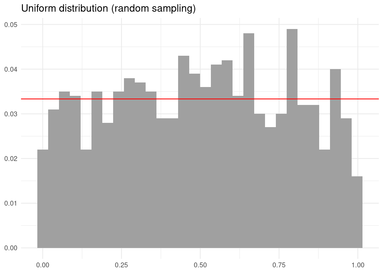

The obtained distribution is quite irregular. We can improve that with lhs::randomLHS(), which has two main inputs:

the number of observations n.
the number of variables k.

The result is a matrix with n rows and k columns. Each column is a stratified sampling of a uniform distribution between zero and one. Let’s see the output of this sampling.

set.seed(111)
lhs_unif_sample <- tibble(obs = randomLHS(1000, 1)[, 1])

lhs_unif_sample |>
  ggplot(aes(obs)) +
  geom_histogram(aes(y = after_stat(count / sum(count))), fill = "#A0A0A0") +
  geom_hline(yintercept = 1/30, color = "red") +
  labs(title = "Uniform distribution (LHS sampling)", x = NULL, y = NULL) +
  theme_minimal()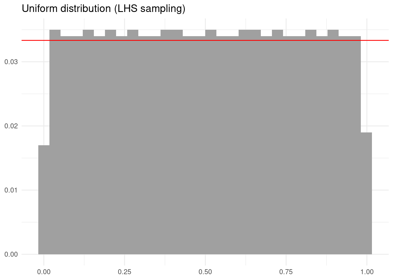

The outcome is a more regular sampling of the uniform probability distribution.

Probability Distributions

If instead of the uniform distribution we simulate the N(0, 1) distribution we also obtain distorted results.

set.seed(444)
norm_sample <- tibble(obs = rnorm(1000))

norm_sample |>
  ggplot(aes(obs)) +
  geom_histogram(aes(y = after_stat(count / sum(count))), fill = "#A0A0A0") +
  geom_hline(yintercept = 1/30, color = "red") +
  labs(title = "Normal distribution (random sampling)", x = NULL, y = NULL) +
  theme_minimal()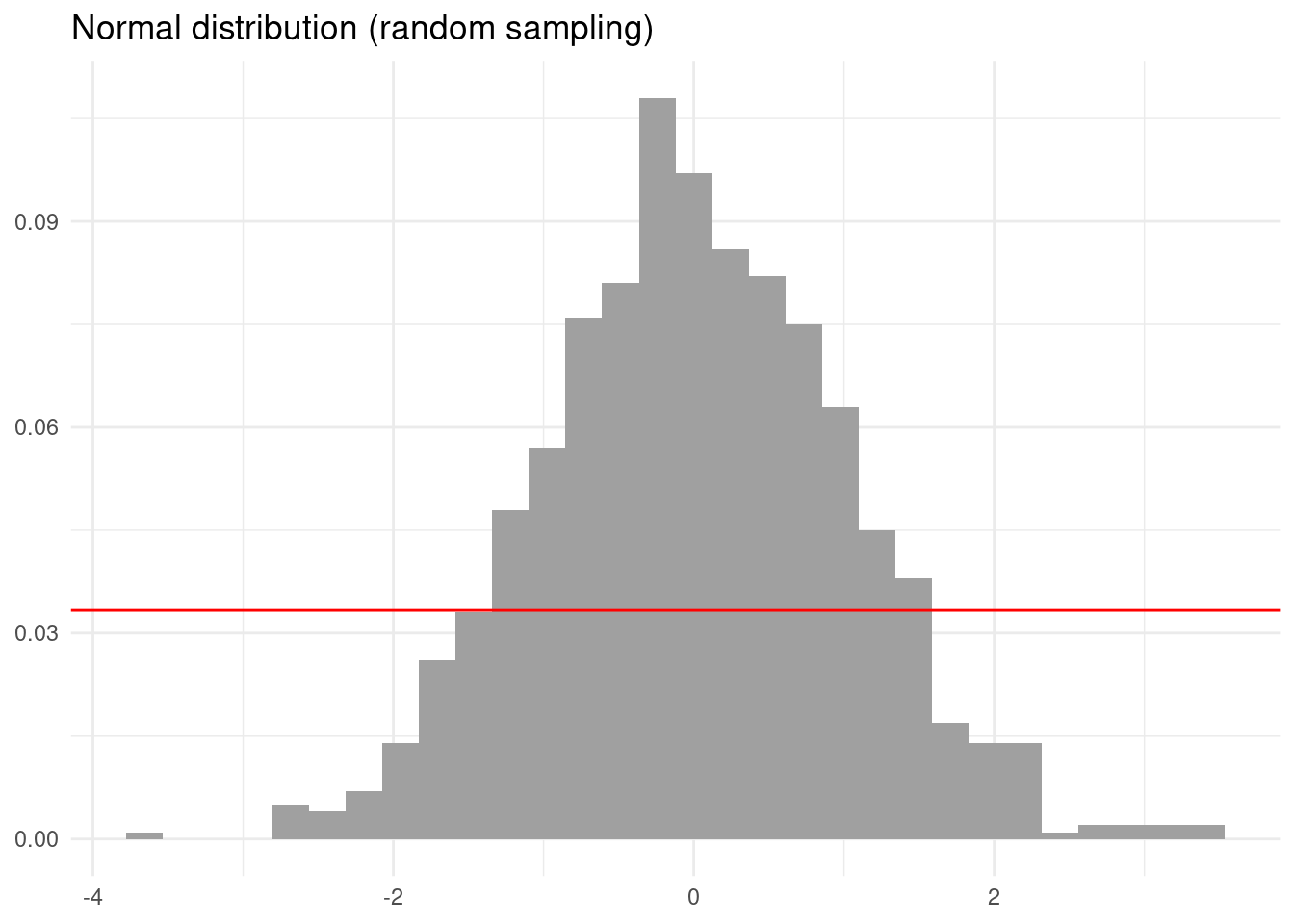

We can generate stratified samples of any probability distribution using functions analogous to the qnorm() function for the normal distribution. This function returns the value of the quantiles of the N(0, 1) distribution. Let’s generate a stratified sampling of a normal distribution doing as follows.

set.seed(444)
lhs_norm_sample <- tibble(u_obs = randomLHS(1000, 1)[, 1]) |>
  mutate(obs = qnorm(u_obs))

lhs_norm_sample |>
  ggplot(aes(obs)) +
  geom_histogram(aes(y = after_stat(count / sum(count))), fill = "#A0A0A0") +
  geom_hline(yintercept = 1/30, color = "red") +
  labs(title = "Normal distribution (LHS sampling)", x = NULL, y = NULL) +
  theme_minimal()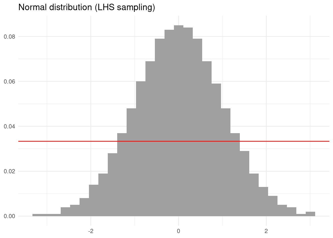

Again the result looks more regular than the simulation with non-stratified sampling.

Multivariate Distribution

Let’s illustrate the principle of the Latin square with a sampling of ten observations:

set.seed(555)
randomLHS(10, 2) |> 
  data.frame() |>
  ggplot(aes(X1, X2)) +
  geom_point() +
  geom_hline(yintercept = seq(0, 1, length.out = 11), color = "#A0A0A0") +
  geom_vline(xintercept = seq(0, 1, length.out = 11), color = "#A0A0A0") +
  theme_minimal() +
  labs(title = "Random Latin square sampling", x = NULL, y = NULL)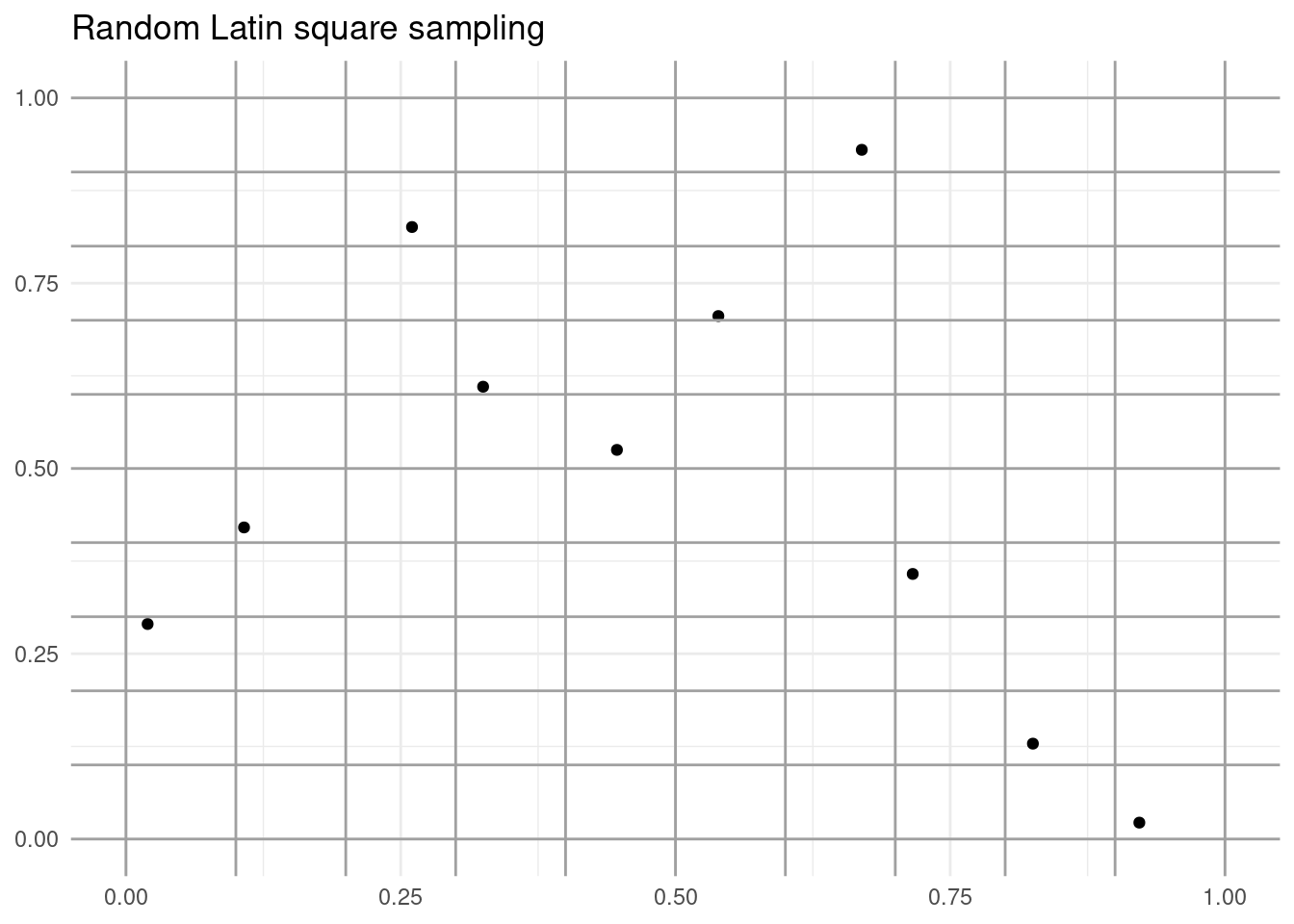

Each row and column of the grid contains a single observation. Thus, we ensure that the correlation between both samples is low.

Let’s generate a multivariate distribution with the following properties:

One variable follows a normal distribution.
A second variable follows a lognormal distribution.
A third variable follows a Pert distribution.
The three variables are uncorrelated.

The code to generate the sample is:

multiv_lhs <- randomLHS(1000, 3) |>
  data.frame()

multiv_lhs <- multiv_lhs |>
  mutate(norm = qnorm(X1),
         lnorm = qlnorm(X2),
         pert = qpert(X3, 1, 4, 5)) |>
  select(norm:pert)

Let’s examine multiv_lhs with GGally::multiv_lhs()

ggpairs(multiv_lhs) +
  theme_linedraw()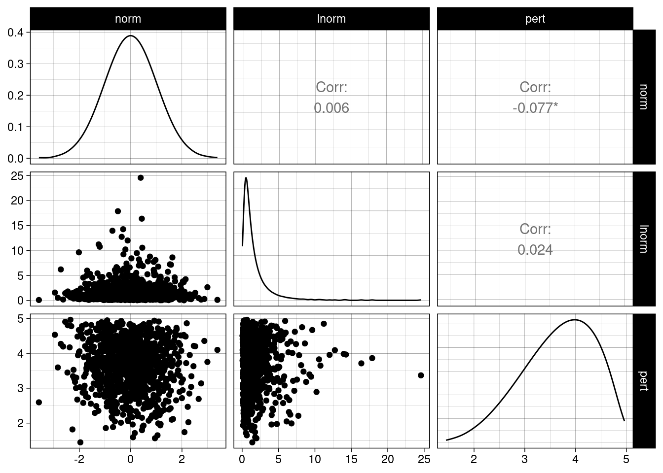

Each of the variables follows the requested distribution, and simultaneously the correlation between variables is small.

Application to Monte Carlo

Let’s examine how the Latin hypercube sampling can help us in a classical elementary application of Monte Carlo consisting in estimating \(\pi\).

To do so, we consider a square with four sides with values ranging between zero and one. The area of the square is equal to 4, and the circle of radius one inscribed in the square has area \(\pi\). Therefore, the probability of an arbitrary point of the square of falling within the circle is \(p = \pi/4\). If we estimate the probability \(p\) with Monte Carlo simulation we can estimate \(\pi\) as \(\pi = 4p\).

We implement this procedure in the pi_mc function, which has two arguments:

the number of observations n.
the method to obtain random numbers eval, which can take two values: "random" for purely random generation, and "lhs" for Latin hypercube sampling.

pi_mc <- function(n, eval = "random"){
  
  if(eval == "random"){
    t <- data.frame(x = runif(n, -1 ,1),
                y = runif(n, -1, 1))
  }
  
  if(eval == "lhs"){
    m <- randomLHS(n, 2)
    m <- apply(m, 2, \(x) x*2 - 1)
    t <- data.frame(m)
    names(t) <- c("x", "y")
  }
  
  t <- t |>
    mutate(inside = ifelse(x^2 + y^2 <= 1, 1, 0))
  
  pi <- 4*mean(t$inside)
  
  return(list(t = t, pi = pi))

}

Let’s see how this estimation operates.

set.seed(33)
pi_estimation <- pi_mc(n = 1000)

The estimation of \(\pi\) obtained is:

pi_estimation$pi

## [1] 3.176

The value of \(\pi\) is estimated as the fraction of blue points falling within the circle times four.

circle <- tibble(grades = seq(0, 2*pi, length.out = 100),
                 x = cos(grades),
                 y = sin(grades))

pi_estimation$t |>
  ggplot(aes(x, y)) +
  geom_point(aes(color = factor(inside)), size = 2) +
  theme_void() +
  geom_path(data = circle, aes(x, y)) +
  theme(legend.position = "none")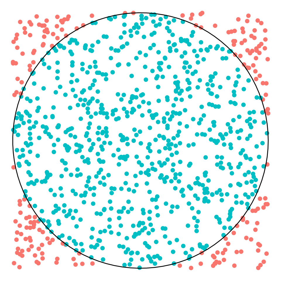

To examine the effect of Latin hypercube sampling, I will run 100 times the simulation with three different numbers of points and the two methods.

set.seed(44)
test <- expand_grid(n = c(100, 1000, 10000), eval = 1:100)

test <- test |>
  mutate(pi_random = map_dbl(n, ~ pi_mc(. , "random")$pi),
         pi_lhs = map_dbl(n, ~ pi_mc(., "lhs")$pi))

The results shows that, while the two sampling methods are unbiaised, meaning that the average across samples is close to \(\pi\), the Latin hypercube sampling method has less variability because of better sampling. This advantage tends to vanish as we use a large number of points to do the estimation.

test |>
  pivot_longer(starts_with("pi")) |>
  ggplot(aes(factor(n), value)) +
    geom_boxplot() +
  geom_hline(yintercept = pi, color = "red", linetype = "dashed") +
    facet_grid(name ~ .) +
  theme_classic(base_size = 12) +
  labs(title = "Finding pi with Monte Carlo", x = "sample size", y = NULL)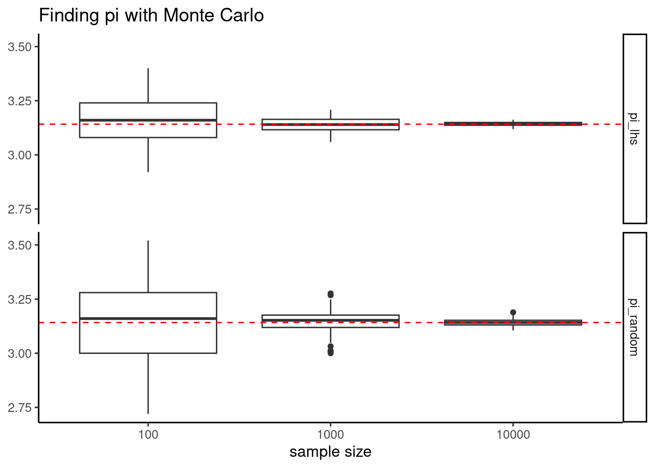

Latin Hypercube Sampling (LHS) is a statistical method for generating a sample of plausible values from a multidimensional distribution. LHS uses stratified sampling to ensure that each parameter is sampled across all ranges of values of the probability distribution. With LHS, we can generate multivariate samples of uncorrelated variables of any probability distribution.

We can use the lhs package to generate LHS samples. The output of this sampling can be used as input of other packages for Monte Carlo simulation like mc2d.

References

Carnieli, R. (2024). Basic Latin hypercube samples and designs with package lhs. https://cran.r-project.org/web/packages/lhs/vignettes/lhs_basics.html. Accessed 26 October 2024.
lhs github page. https://bertcarnell.github.io/lhs/. Accessed 26 October 2024.

The introduction to the Latin hypercube sampling is an edition of a ChatGPT text.

Session Info

sessionInfo()

## R version 4.4.1 (2024-06-14)
## Platform: x86_64-pc-linux-gnu
## Running under: Linux Mint 21.1
## 
## Matrix products: default
## BLAS:   /usr/lib/x86_64-linux-gnu/blas/libblas.so.3.10.0 
## LAPACK: /usr/lib/x86_64-linux-gnu/lapack/liblapack.so.3.10.0
## 
## locale:
##  [1] LC_CTYPE=es_ES.UTF-8       LC_NUMERIC=C              
##  [3] LC_TIME=es_ES.UTF-8        LC_COLLATE=es_ES.UTF-8    
##  [5] LC_MONETARY=es_ES.UTF-8    LC_MESSAGES=es_ES.UTF-8   
##  [7] LC_PAPER=es_ES.UTF-8       LC_NAME=C                 
##  [9] LC_ADDRESS=C               LC_TELEPHONE=C            
## [11] LC_MEASUREMENT=es_ES.UTF-8 LC_IDENTIFICATION=C       
## 
## time zone: Europe/Madrid
## tzcode source: system (glibc)
## 
## attached base packages:
## [1] stats     graphics  grDevices utils     datasets  methods   base     
## 
## other attached packages:
##  [1] mc2d_0.2.1      mvtnorm_1.2-5   GGally_2.2.1    lhs_1.2.0      
##  [5] lubridate_1.9.3 forcats_1.0.0   stringr_1.5.1   dplyr_1.1.4    
##  [9] purrr_1.0.2     readr_2.1.5     tidyr_1.3.1     tibble_3.2.1   
## [13] ggplot2_3.5.1   tidyverse_2.0.0
## 
## loaded via a namespace (and not attached):
##  [1] sass_0.4.9         utf8_1.2.4         generics_0.1.3     rstatix_0.7.2     
##  [5] blogdown_1.19      stringi_1.8.3      hms_1.1.3          digest_0.6.35     
##  [9] magrittr_2.0.3     evaluate_0.23      grid_4.4.1         timechange_0.3.0  
## [13] RColorBrewer_1.1-3 bookdown_0.39      fastmap_1.1.1      plyr_1.8.9        
## [17] jsonlite_1.8.8     backports_1.4.1    fansi_1.0.6        scales_1.3.0      
## [21] jquerylib_0.1.4    abind_1.4-5        cli_3.6.2          rlang_1.1.3       
## [25] munsell_0.5.1      withr_3.0.0        cachem_1.0.8       yaml_2.3.8        
## [29] tools_4.4.1        tzdb_0.4.0         ggsignif_0.6.4     colorspace_2.1-0  
## [33] ggpubr_0.6.0       ggstats_0.7.0      broom_1.0.5        vctrs_0.6.5       
## [37] R6_2.5.1           lifecycle_1.0.4    car_3.1-2          pkgconfig_2.0.3   
## [41] pillar_1.9.0       bslib_0.7.0        gtable_0.3.5       glue_1.7.0        
## [45] Rcpp_1.0.12        highr_0.10         xfun_0.43          tidyselect_1.2.1  
## [49] rstudioapi_0.16.0  knitr_1.46         farver_2.1.1       htmltools_0.5.8.1 
## [53] labeling_0.4.3     carData_3.0-5      rmarkdown_2.26     compiler_4.4.1

The Jose M Sallan static website