Cluster analysis, or clustering, is a data analysis technique aimed at partitioning a set of objects into groups such that objects within the same group or cluster exhibit greater similarity to one another than to those in other groups. One of the best known clustering techniques is k-means clustering. The aim of k-means clustering is to minimize the sum of within-clusters sum of squares. Objects are assigned to the cluster whose centroid is closer to the object. Usually k-means is implemented through a iterative heuristic. In R, this heuristic is implemented in the kmeans() R base function.
In this post, I will present an example of k-means clustering with geographical data, using the set of nightlife venues of Barcelona registered in 2024. Additionnally I will show how can we extract information from kmeans() using broom, how to obtain a reasonable value of the number of clusters \(k\) and how to interpret the results using data features, in this case the neoighbourhood where venues are located.
library(tidyverse)
library(broom)
library(sf)
library(BAdatasetsSpatial)
library(kselection)
Data
There are two relevant datasets for this analysis. First I will retrieve a Barcelona neighborhood map bcn_neigh from BAdatasetsSpatial.
bcn_neigh <- BCNNeigh |>
  select(c_barri, n_barri, c_distri, n_distri)
Second I will retrieve relevant information from each venue, specifically the geographical location with longitud and latitud, the neighborhood and the name and address. All is gathered in the nightlife_2024 data frame.
nightlife_2024 <- data_2024 |>
  select(nom_local, latitud, longitud, nom_barri, codi_barri, nom_via, porta)
Now I need to elaborate on this data a bit more. Instead of relying on dataset information, I will perform a spatial join to assign the neighborhood to each venue. To do so, I need to create the simple feature object nightlife_2024_sf and then do the spatial join with bcn_neigh.
nightlife_2024_sf <- nightlife_2024 |>
  st_as_sf(coords = c("longitud", "latitud"), crs = 4326, remove = FALSE)

nightlife_2024_sf  <- st_join(nightlife_2024_sf,
                              bcn_neigh |> select(c_barri, n_barri),
                              join = st_intersects)
Finally, I am removing observations that fall out of the polygons of bcn_neigh.
nightlife_2024_sf <- nightlife_2024_sf |>
  filter(!is.na(c_barri))
k-means Clustering with broom
Let’s test how the kmeans() function works. In this case, we are using as features longitude and latitude. In this case, the distance between observations can be interpreted as geographical distance. First we need to prepare the nl_coords table retaining the relevant variables and removing the geometry column.
nl_coords <- nightlife_2024_sf |>
  st_drop_geometry() |>
  select(longitud, latitud)
Let’s do a k-means clustering with four centers. As the heuristics has random elements, I am setting a seed of random numbers for reproducibility. The result of the analysis is stored in test_kmeans.
set.seed(55)
test_kmeans <- kmeans(nl_coords, centers = 4)
Let’s apply the three functions of broom to test_kemans.
tidy(test_kmeans) # centers of clusters## # A tibble: 4 × 5
## longitud latitud size withinss cluster
## <dbl> <dbl> <int> <dbl> <fct>
## 1 2.16 41.4 54 0.00403 1
## 2 2.14 41.4 77 0.0125 2
## 3 2.18 41.4 63 0.00541 3
## 4 2.17 41.4 47 0.0119 4glance(test_kmeans) # performance metrics## # A tibble: 1 × 4
## totss tot.withinss betweenss iter
## <dbl> <dbl> <dbl> <int>
## 1 0.128 0.0338 0.0938 3augment(test_kmeans, data = nl_coords) # assigns cluster variable## # A tibble: 241 × 3
## longitud latitud .cluster
## <dbl> <dbl> <fct>
## 1 2.15 41.4 2
## 2 2.13 41.4 2
## 3 2.16 41.4 1
## 4 2.14 41.4 2
## 5 2.17 41.4 1
## 6 2.17 41.4 1
## 7 2.15 41.4 2
## 8 2.17 41.4 1
## 9 2.17 41.4 4
## 10 2.13 41.4 2
## # ℹ 231 more rowsFor k-means clustering the broom functions retrieve the following information:
tidy()returns the centroids of each of the clusters.glance()presents some performance parameters. The more relevant is the within-clusters sum of squarestot.withinss.augment()adds todataa.clustercolumn with the cluster assigned to each observation. For convenience, this column is encoded as factor.
I have used augment() and tidy() to plot the solution of the clustering with four centers, representing each point and the clusters centroids.
augment(test_kmeans, data = nl_coords) |>
  ggplot(aes(longitud, latitud, color = .cluster)) +
  geom_point() +
  geom_point(data = tidy(test_kmeans), aes(longitud, latitud, color = cluster), shape = 3, size = 10) +
  theme_minimal() +
  theme(legend.position = "none")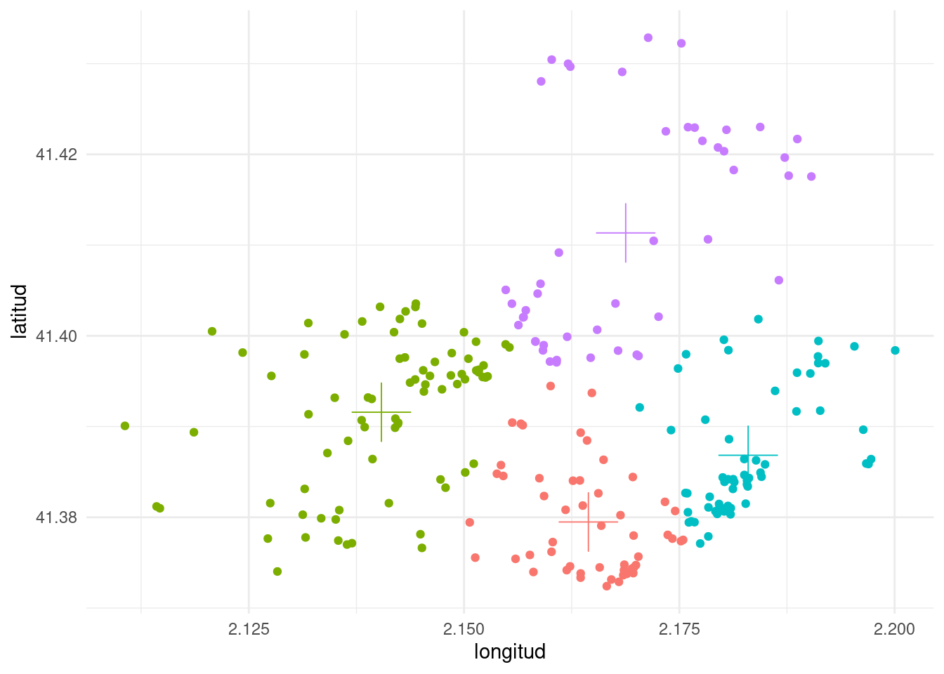
From the plot, we observe that the clusters obtained with k-means tend to be of circular shape, centered in the cluster centroid.
Number of Clusters
It is about time to select how many clusters to enter into the k-means algorithm. The first strategy is to evaluate the within-clusters sum of squares for a range of values of k. As k increases the sum of squares is smaller, but there is a moment where the gain of performance is not significant. We can appreciate that plotting the within-clusters sum of squares versus the number of clusters. The elbow_table contains the performance metrics obtained with glance() for values of k between one and ten.
set.seed(1111)
elbow_table <-
  map_dfr(1:10, ~ kmeans(nl_coords, centers = .) |>
            glance() |>
            mutate(k = .) |>
            relocate(k))

elbow_table |>
  ggplot(aes(k, tot.withinss)) +
  geom_line() +
  geom_point() +
  geom_vline(xintercept = 5, linetype = "dashed",
             color ="red", linewidth = 1) +
  scale_x_continuous(breaks = 1:10) +
  theme_minimal(base_size = 12)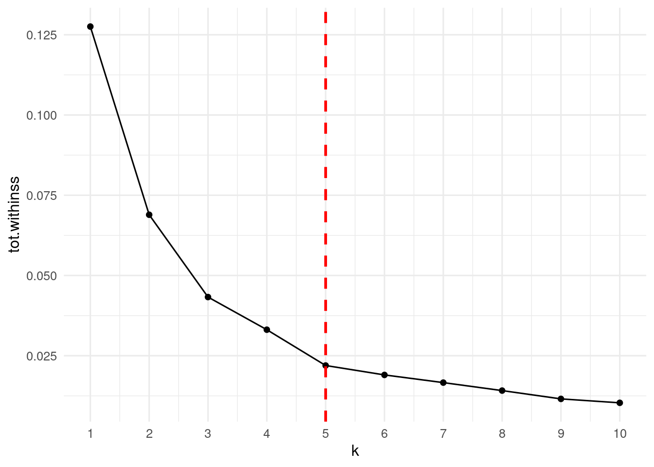
From the plot above, the elbow point from which within-clusters sum of squares is not reduced significantly is k = 5.
The kselection package implements the procedure described by Pahm et al. (2004) to determine the number of clusters in k-means clustering. Here I have just run the code presented in the package vignette.
set.seed(1313)
sol <- kselection(nl_coords)
num_clusters(sol)
## [1] 13get_f_k(sol)## [1] 1.0000000 0.8644771 0.9132815 1.0342962 0.8466897 1.0194538 0.9463159
## [8] 0.9961763 1.0007176 0.9894164 1.0666465 0.9523737 0.7859992 1.0725217
## [15] 0.8699234plot(sol)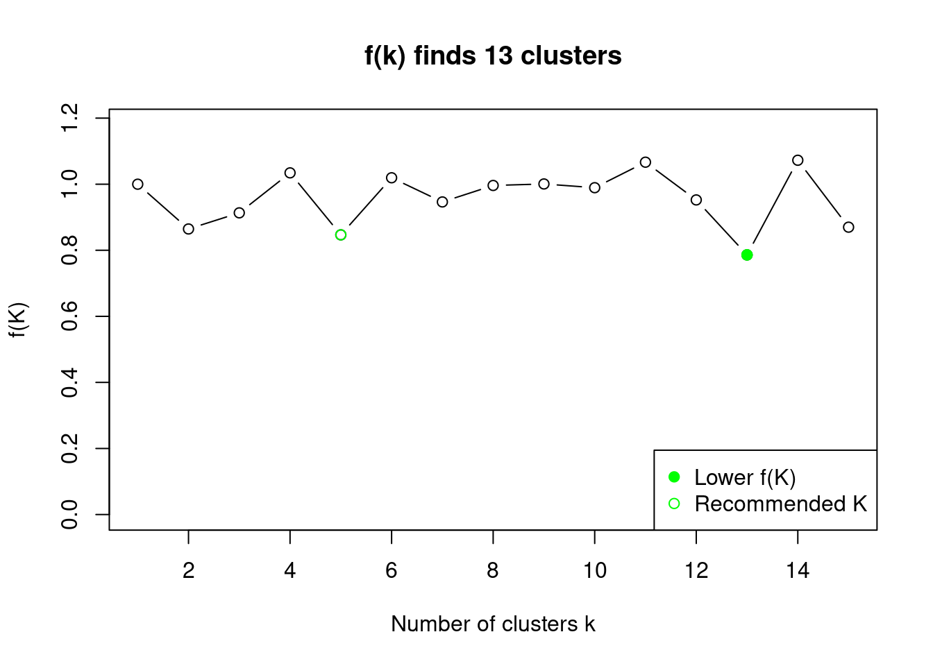
kselection recommends also k = 5 clusters.
Five Nightlife Clusters
Let’s find the k-means partition of nightlife venues into five clusters. The result is in nl_kmeans05.
set.seed(1212)
nl_kmeans_05 <- kmeans(nl_coords, centers = 5)
I am adding the cluster variable to nightlife_2024_sf as a vector. I cannot use glance() here, as it does not work with spatial objects.
nightlife_2024_sf <- nightlife_2024_sf |>
  mutate(cluster = as.factor(nl_kmeans_05$cluster)) # augment() cannot be used
Let’s do a draft of the map with the venues colored by cluster.
ggplot(bcn_neigh) +
  geom_sf() +
  geom_sf(data = nightlife_2024_sf, aes(color = cluster))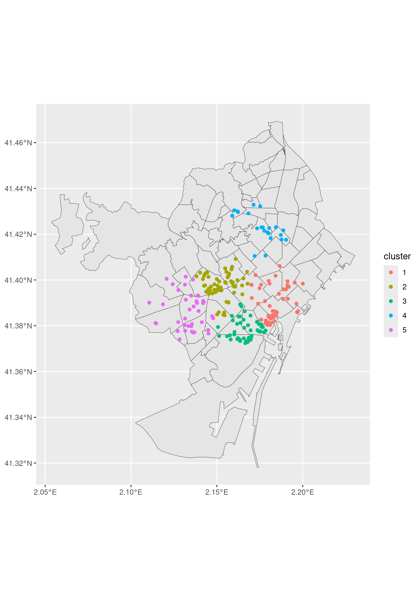
Interpreting Clusters
To interpret the clusters, I will count the number of venues by cluster and neighborhood. The results are in the clusters_neigh table.
clusters_neigh <- nightlife_2024_sf |>
  st_drop_geometry() |>
  group_by(cluster, n_barri) |>
  summarise(venues = n(), .groups = "drop")
Let’s examine clusters one by one:
clusters_neigh |>
  filter(cluster == 1) # gotic - la ribera
## # A tibble: 9 × 3
## cluster n_barri venues
## <fct> <chr> <int>
## 1 1 Sant Pere, Santa Caterina i la Ribera 16
## 2 1 el Barri Gòtic 21
## 3 1 el Clot 1
## 4 1 el Fort Pienc 3
## 5 1 el Parc i la Llacuna del Poblenou 8
## 6 1 el Poblenou 1
## 7 1 la Barceloneta 3
## 8 1 la Dreta de l'Eixample 6
## 9 1 la Vila Olímpica del Poblenou 2clusters_neigh |>
filter(cluster == 2) # sant gervasi - gracia## # A tibble: 6 × 3
## cluster n_barri venues
## <fct> <chr> <int>
## 1 2 Sant Gervasi - Galvany 29
## 2 2 el Camp d'en Grassot i Gràcia Nova 1
## 3 2 l'Antiga Esquerra de l'Eixample 8
## 4 2 la Dreta de l'Eixample 8
## 5 2 la Nova Esquerra de l'Eixample 5
## 6 2 la Vila de Gràcia 15clusters_neigh |>
filter(cluster == 3) #poble sec and raval, lower Eixample## # A tibble: 6 × 3
## cluster n_barri venues
## <fct> <chr> <int>
## 1 3 Sant Antoni 7
## 2 3 el Barri Gòtic 2
## 3 3 el Poble Sec 23
## 4 3 el Raval 16
## 5 3 l'Antiga Esquerra de l'Eixample 3
## 6 3 la Nova Esquerra de l'Eixample 1clusters_neigh |>
filter(cluster == 4) # guinardo - horta## # A tibble: 10 × 3
## cluster n_barri venues
## <fct> <chr> <int>
## 1 4 Horta 3
## 2 4 Navas 3
## 3 4 Vilapicina i la Torre Llobeta 1
## 4 4 el Baix Guinardó 1
## 5 4 el Carmel 1
## 6 4 el Congrés i els Indians 1
## 7 4 el Guinardó 8
## 8 4 el Turó de la Peira 2
## 9 4 la Sagrada Família 1
## 10 4 la Sagrera 1clusters_neigh |>
filter(cluster == 5) # sants and les corts // covers also Sarrià and Les Tres Torres## # A tibble: 10 × 3
## cluster n_barri venues
## <fct> <chr> <int>
## 1 5 Hostafrancs 2
## 2 5 Pedralbes 2
## 3 5 Sant Gervasi - Galvany 3
## 4 5 Sants 9
## 5 5 Sants - Badal 2
## 6 5 Sarrià 3
## 7 5 la Maternitat i Sant Ramon 3
## 8 5 la Nova Esquerra de l'Eixample 2
## 9 5 les Corts 11
## 10 5 les Tres Torres 3The five clusters can be interpreted as follows:
- Cluster 1 Gòtic - la Ribera. A cluster covering the north of the city centre. Also covers venues of close neighborhoods, extening to Port Olímpic.
- Cluster 2 Sant Gervasi - Gràcia. Venues above the Diagonal street, more focused on a local, affluent public.
- Cluster 3 Poble Sec - Raval: Venues of the south of the city centre. While Raval venues are targeted to tourists, Poble Sec honors a lasting tradition of nightlife.
- Cluster 4 Guinardó - Horta: This part of the city comes from villages that were absorbed by Barcelona, and that they have still their own communities. The most relevant nightlife scenes are from Guinardó, Horta and Navas.
- Cluster 5 Les Corts - Sarrià: even more posh than Sant Gervasi, this cluster covers the nightlife of the richest neighbourhoods.
The Five Nightlife Clusters
Here is the map of the five nightlife clusters, with some coloring and the clusters labels.
ggplot(bcn_neigh) +
  geom_sf(fill = "#FFE5CC") +
  geom_sf(data = nightlife_2024_sf, aes(color = cluster)) +
  scale_color_brewer(labels = c("Gòtic - la Ribera", "Sant Gervasi - Gràcia", "Poble Sec - Raval", "Guinardó - Horta",  "Les Corts - Sarrià"),
                     palette = "Dark2") +
  theme_void() +
  theme(legend.position = "inside",
        legend.position.inside = c(0.2, 0.3),
        panel.background = element_rect(fill = "white"))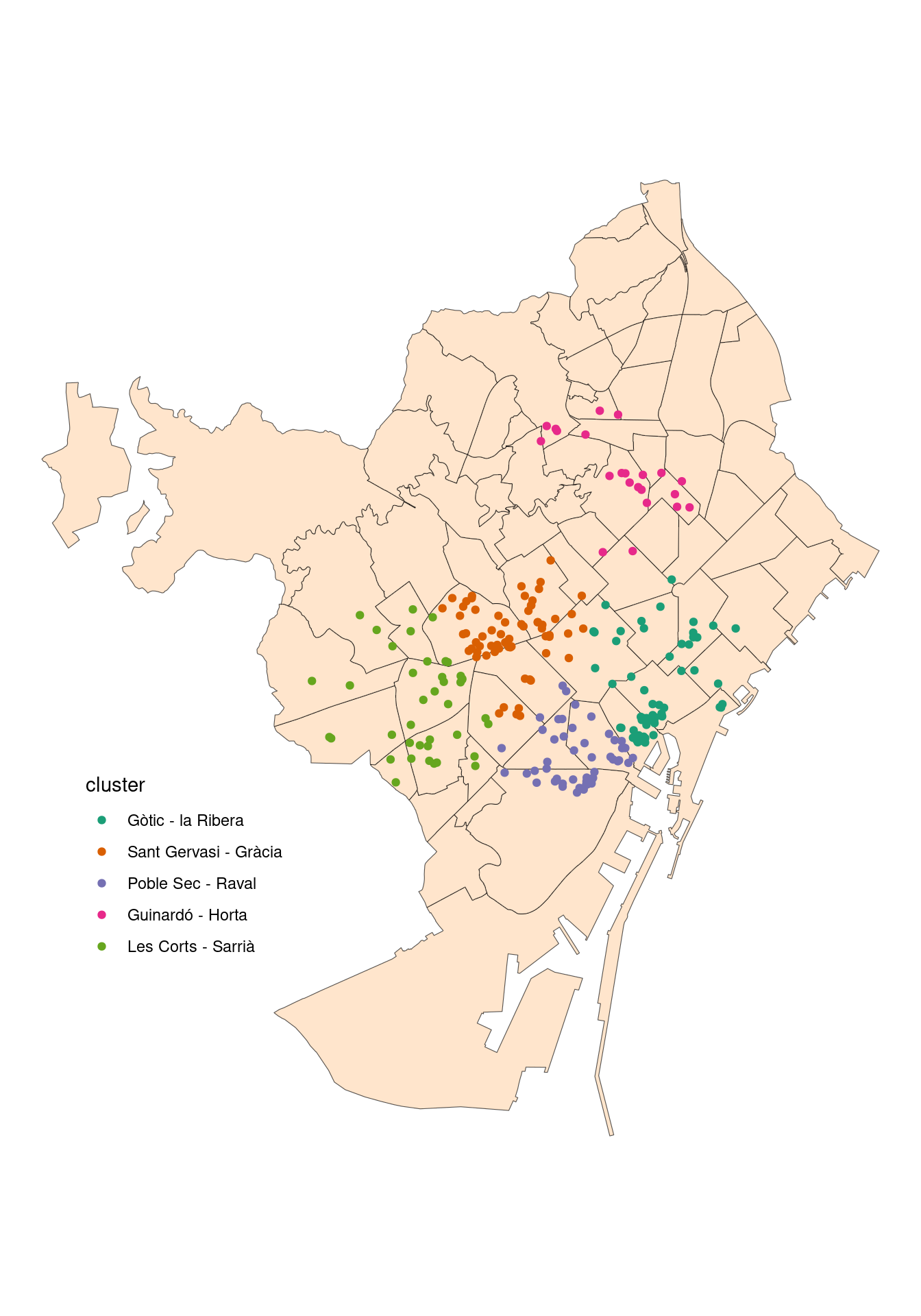
As elements are added to the cluster by proximity to cluster centroid, these tend to be circular. This can be overriden by other clustering algorithms like DBSCAN.
References
- Package
kselection: https://github.com/drodriguezperez/kselection - D T Pham, S S Dimov, and C D Nguyen (2004). Selection of k in k-means clustering, Mechanical Engineering Science, 219(1), 103-119. https://doi.org/10.1243/095440605X8298
Session Info
## R version 4.5.2 (2025-10-31)
## Platform: x86_64-pc-linux-gnu
## Running under: Linux Mint 21.1
##
## Matrix products: default
## BLAS:   /usr/lib/x86_64-linux-gnu/blas/libblas.so.3.10.0
## LAPACK: /usr/lib/x86_64-linux-gnu/lapack/liblapack.so.3.10.0  LAPACK version 3.10.0
##
## locale:
##  [1] LC_CTYPE=es_ES.UTF-8       LC_NUMERIC=C
##  [3] LC_TIME=es_ES.UTF-8        LC_COLLATE=es_ES.UTF-8
##  [5] LC_MONETARY=es_ES.UTF-8    LC_MESSAGES=es_ES.UTF-8
##  [7] LC_PAPER=es_ES.UTF-8       LC_NAME=C
##  [9] LC_ADDRESS=C               LC_TELEPHONE=C
## [11] LC_MEASUREMENT=es_ES.UTF-8 LC_IDENTIFICATION=C
##
## time zone: Europe/Madrid
## tzcode source: system (glibc)
##
## attached base packages:
## [1] stats     graphics  grDevices utils     datasets  methods   base
##
## other attached packages:
##  [1] kselection_0.2.1        BAdatasetsSpatial_0.1.0 sf_1.0-20
##  [4] broom_1.0.10            lubridate_1.9.4         forcats_1.0.1
##  [7] stringr_1.6.0           dplyr_1.1.4             purrr_1.2.0
## [10] readr_2.1.5             tidyr_1.3.1             tibble_3.3.0
## [13] ggplot2_4.0.0           tidyverse_2.0.0
##
## loaded via a namespace (and not attached):
##  [1] s2_1.1.7           utf8_1.2.4         sass_0.4.10        generics_0.1.3
##  [5] class_7.3-23       KernSmooth_2.23-26 blogdown_1.21      stringi_1.8.7
##  [9] hms_1.1.4          digest_0.6.37      magrittr_2.0.4     evaluate_1.0.3
## [13] grid_4.5.2         timechange_0.3.0   RColorBrewer_1.1-3 bookdown_0.43
## [17] fastmap_1.2.0      jsonlite_2.0.0     e1071_1.7-16       backports_1.5.0
## [21] DBI_1.2.3          scales_1.4.0       jquerylib_0.1.4    cli_3.6.4
## [25] rlang_1.1.6        units_0.8-7        withr_3.0.2        cachem_1.1.0
## [29] yaml_2.3.10        tools_4.5.2        tzdb_0.5.0         vctrs_0.6.5
## [33] R6_2.6.1           proxy_0.4-27       lifecycle_1.0.4    classInt_0.4-11
## [37] pkgconfig_2.0.3    pillar_1.11.1      bslib_0.9.0        gtable_0.3.6
## [41] Rcpp_1.1.0         glue_1.8.0         xfun_0.52          tidyselect_1.2.1
## [45] rstudioapi_0.17.1  knitr_1.50         farver_2.1.2       htmltools_0.5.8.1
## [49] labeling_0.4.3     rmarkdown_2.29     wk_0.9.4           compiler_4.5.2
## [53] S7_0.2.0