The dplyr package for tabular data handling includes a set of functions for joining data frames with a relational structure. By relational structure, I mean that there are columns in each table that can relate the contents of the two tables.
I will illustrate how these functions work using data from the World Bank. In addition to dplyr, I am using the wbstats package to retrieve those data directly from the web.
library(dplyr)
library(wbstats)
Mutating joins (also called merges) return a data frame with the columns of two data frames x and y:
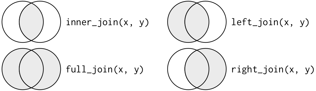
inner join: returns all rows from x where there are matching values in y. If there are multiple matches between x and y, all combination of the matches are returned.
full (outer) join: returns all rows from both x and y. Where there are not matching values, returns NA for the ones missing.
left join: returns all rows from x. Rows of x with no match in y will have NA values in the y columns. If there are multiple matches between x and y, all combination of the matches are returned.
right join: returns all rows from y. Rows of y with no match in x will have
NAvalues in the x columns. If there are multiple matches, all combinations are returned.
These four mutating joins are implemented in dplyr with the functions inner_join, full_join, left_join and right_join.
Getting data from the World Bank
Let’s use the wbstats package to retrieve values of two series:
- The
SP.POP.TOTLindicator of total population https://data.worldbank.org/indicator/SP.POP.TOTL - The
SP.DYN.TFRT.INof total fertility rate in rates per woman https://data.worldbank.org/indicator/SP.DYN.TFRT.IN
pop_wb <- wb_data("SP.POP.TOTL", start_date = 2000, end_date = 2022)
pop_wb
## # A tibble: 4,557 × 9
## iso2c iso3c country date SP.POP.TOTL unit obs_status footnote last_updated
## <chr> <chr> <chr> <dbl> <dbl> <chr> <chr> <chr> <date>
## 1 AF AFG Afghani… 2020 38928341 <NA> <NA> <NA> 2022-02-15
## 2 AF AFG Afghani… 2019 38041757 <NA> <NA> <NA> 2022-02-15
## 3 AF AFG Afghani… 2018 37171922 <NA> <NA> <NA> 2022-02-15
## 4 AF AFG Afghani… 2017 36296111 <NA> <NA> <NA> 2022-02-15
## 5 AF AFG Afghani… 2016 35383028 <NA> <NA> <NA> 2022-02-15
## 6 AF AFG Afghani… 2015 34413603 <NA> <NA> <NA> 2022-02-15
## 7 AF AFG Afghani… 2014 33370804 <NA> <NA> <NA> 2022-02-15
## 8 AF AFG Afghani… 2013 32269592 <NA> <NA> <NA> 2022-02-15
## 9 AF AFG Afghani… 2012 31161378 <NA> <NA> <NA> 2022-02-15
## 10 AF AFG Afghani… 2011 30117411 <NA> <NA> <NA> 2022-02-15
## # … with 4,547 more rowstfrt_wb <- wb_data("SP.DYN.TFRT.IN", start_date = 2000, end_date = 2022)
tfrt_wb## # A tibble: 4,557 × 9
## iso2c iso3c country date SP.DYN.TFRT.IN unit obs_status footnote
## <chr> <chr> <chr> <dbl> <dbl> <chr> <chr> <chr>
## 1 AW ABW Aruba 2000 1.87 <NA> <NA> <NA>
## 2 AW ABW Aruba 2001 1.85 <NA> <NA> <NA>
## 3 AW ABW Aruba 2002 1.82 <NA> <NA> <NA>
## 4 AW ABW Aruba 2003 1.80 <NA> <NA> <NA>
## 5 AW ABW Aruba 2004 1.79 <NA> <NA> <NA>
## 6 AW ABW Aruba 2005 1.77 <NA> <NA> <NA>
## 7 AW ABW Aruba 2006 1.76 <NA> <NA> <NA>
## 8 AW ABW Aruba 2007 1.76 <NA> <NA> <NA>
## 9 AW ABW Aruba 2008 1.76 <NA> <NA> <NA>
## 10 AW ABW Aruba 2009 1.76 <NA> <NA> <NA>
## # … with 4,547 more rows, and 1 more variable: last_updated <date>I will edit the resulting tables removing missing values, retaining the columns with country, date and value and renaming the value.
pop <- pop_wb %>%
  filter(!is.na(SP.POP.TOTL)) %>%
  select(country, date, SP.POP.TOTL) %>%
  rename(population = SP.POP.TOTL)

tfrt <- tfrt_wb %>%
  filter(!is.na(SP.DYN.TFRT.IN)) %>%
  select(country, date, SP.DYN.TFRT.IN) %>%
  rename(fertility = SP.DYN.TFRT.IN)
Joins by one variable
I will start joining tables with data from year 2010:
pop_2010 <- pop %>%
  filter(date == 2010) %>%
  select(-date)

tfrt_2010 <- tfrt %>%
  filter(date == 2010) %>%
  select(-date)
Both tables have different number of observations:
pop_2010has 217 rows.tfrt_2010has 201 rows.
It is important to track the number of rows of each table to examine the effect of each join. Let’s begin with the inner join. Like in the rest of joins, I have declared the joining columns with by. If no value of by is passed, the functions pick the columns of equal name in both tables.
inner_2010 <- inner_join(pop_2010,
                         tfrt_2010,
                         by = "country")
inner_2010
## # A tibble: 201 × 3
## country population fertility
## <chr> <dbl> <dbl>
## 1 Afghanistan 29185511 5.98
## 2 Albania 2913021 1.66
## 3 Algeria 35977451 2.86
## 4 Andorra 84454 1.27
## 5 Angola 23356247 6.19
## 6 Antigua and Barbuda 88030 1.99
## 7 Argentina 40788453 2.35
## 8 Armenia 2877314 1.72
## 9 Aruba 101665 1.77
## 10 Australia 22031750 1.93
## # … with 191 more rowsThe inner join will have the least rows of all joins, as it only includes values of the joining columns present in both tables. It has 201 rows, the same as tfrt_2010.
full_2010 <- full_join(pop_2010,
                       tfrt_2010,
                       by = "country")
full_2010
## # A tibble: 217 × 3
## country population fertility
## <chr> <dbl> <dbl>
## 1 Afghanistan 29185511 5.98
## 2 Albania 2913021 1.66
## 3 Algeria 35977451 2.86
## 4 American Samoa 56084 NA
## 5 Andorra 84454 1.27
## 6 Angola 23356247 6.19
## 7 Antigua and Barbuda 88030 1.99
## 8 Argentina 40788453 2.35
## 9 Armenia 2877314 1.72
## 10 Aruba 101665 1.77
## # … with 207 more rowsThe full join has the maximum value of rows of all joins, as it includes the observations included in any of the tables. It has 201 rows, the same as pop_2010.
With the full join, we can examine which rows do not include fertility or population:
full_2010 %>%
  filter(is.na(fertility))
## # A tibble: 16 × 3
## country population fertility
## <chr> <dbl> <dbl>
## 1 American Samoa 56084 NA
## 2 British Virgin Islands 27796 NA
## 3 Cayman Islands 56672 NA
## 4 Dominica 70877 NA
## 5 Gibraltar 33585 NA
## 6 Isle of Man 84856 NA
## 7 Marshall Islands 56361 NA
## 8 Monaco 35609 NA
## 9 Nauru 10009 NA
## 10 Northern Mariana Islands 53971 NA
## 11 Palau 17954 NA
## 12 San Marino 31221 NA
## 13 Sint Maarten (Dutch part) 34056 NA
## 14 St. Kitts and Nevis 49011 NA
## 15 Turks and Caicos Islands 32658 NA
## 16 Tuvalu 10521 NAfull_2010 %>%
filter(is.na(population))## # A tibble: 0 × 3
## # … with 3 variables: country <chr>, population <dbl>, fertility <dbl>We observe that some countries that have populations have not fertility rate records, but not in reverse.
Left and rigth joins will have the same rows of the left and right tables in the join expression, respectively.
left_2010 <- left_join(pop_2010,
                       tfrt_2010,
                       by = "country")
left_2010
## # A tibble: 217 × 3
## country population fertility
## <chr> <dbl> <dbl>
## 1 Afghanistan 29185511 5.98
## 2 Albania 2913021 1.66
## 3 Algeria 35977451 2.86
## 4 American Samoa 56084 NA
## 5 Andorra 84454 1.27
## 6 Angola 23356247 6.19
## 7 Antigua and Barbuda 88030 1.99
## 8 Argentina 40788453 2.35
## 9 Armenia 2877314 1.72
## 10 Aruba 101665 1.77
## # … with 207 more rowsright_2010 <- right_join(pop_2010,
tfrt_2010,
by = "country")
right_2010## # A tibble: 201 × 3
## country population fertility
## <chr> <dbl> <dbl>
## 1 Afghanistan 29185511 5.98
## 2 Albania 2913021 1.66
## 3 Algeria 35977451 2.86
## 4 Andorra 84454 1.27
## 5 Angola 23356247 6.19
## 6 Antigua and Barbuda 88030 1.99
## 7 Argentina 40788453 2.35
## 8 Armenia 2877314 1.72
## 9 Aruba 101665 1.77
## 10 Australia 22031750 1.93
## # … with 191 more rowsJoins by two variables
Let’s join the two original pop and tfrt tables. We need to do the join by two variables: country and year.
inner <- inner_join(pop,
                    tfrt,
                    by = c("country", "date"))

full <- full_join(pop,
                  tfrt,
                  by = c("country", "date"))

left <- left_join(pop,
                  tfrt,
                  by = c("country", "date"))

right <- right_join(pop,
                    tfrt,
                    by = c("country", "date"))
Let’s see how many rows we have in each join and the two original tables:
| table | number of rows |
|---|---|
| pop | 4548 |
| tfrt | 4017 |
| inner | 4009 |
| full | 4556 |
| left | 4548 |
| right | 4017 |
Now the inner table has less rows than tfrt, while the full table has more rows than pop. This means that there are observations in pop missing in tfrt, and vice versa.
Filtering join
To check which observations of one table are missing in the other, we can use the anti_join filtering join: anti_join(x, y) returns observations of x with no match in y.
We can see which elements of pop are not present in tfrt doing:
anti_join(pop, tfrt, by = c("country", "date"))## # A tibble: 539 × 3
## country date population
## <chr> <dbl> <dbl>
## 1 Afghanistan 2020 38928341
## 2 Albania 2020 2837743
## 3 Algeria 2020 43851043
## 4 American Samoa 2020 55197
## 5 American Samoa 2019 55312
## 6 American Samoa 2018 55461
## 7 American Samoa 2017 55617
## 8 American Samoa 2016 55739
## 9 American Samoa 2015 55806
## 10 American Samoa 2014 55791
## # … with 529 more rowsWe have 539 observations in this table. This is not surprising, as fertility records and not as exhaustive as population’s.
Let’s examine which elements of tfrt are not present in pop:
anti_join(tfrt, pop, by = c("country", "date"))## # A tibble: 8 × 3
## country date fertility
## <chr> <dbl> <dbl>
## 1 Eritrea 2012 4.41
## 2 Eritrea 2013 4.34
## 3 Eritrea 2014 4.27
## 4 Eritrea 2015 4.22
## 5 Eritrea 2016 4.16
## 6 Eritrea 2017 4.11
## 7 Eritrea 2018 4.06
## 8 Eritrea 2019 4.00Here we have only 8 observations. None of them is from year 2010, so we did not observed them in the previous section.
dplyr offers a set of functions to join relational tables that allow performing mutating joins, because they return a new table with information from the two inputs. This allows doing SQL-like operations inside the R environment. The four mutating joins (inner, full, left and right) are a replacement for the R base merge function, hopefully in a more intuitive fashion. Filtering joins allow controlling for which rows have no match in the other table, so they do not return a new table.
References
- Filtering joins. https://dplyr.tidyverse.org/reference/filter-joins.html
- Mutating joins. https://dplyr.tidyverse.org/reference/mutate-joins.html
wbstats: An R package for searching and downloading data from the World Bank API. https://cran.r-project.org/web/packages/wbstats/vignettes/wbstats.html
Session info
## R version 4.1.3 (2022-03-10)
## Platform: x86_64-pc-linux-gnu (64-bit)
## Running under: Debian GNU/Linux 10 (buster)
##
## Matrix products: default
## BLAS:   /usr/lib/x86_64-linux-gnu/blas/libblas.so.3.8.0
## LAPACK: /usr/lib/x86_64-linux-gnu/lapack/liblapack.so.3.8.0
##
## locale:
##  [1] LC_CTYPE=es_ES.UTF-8       LC_NUMERIC=C
##  [3] LC_TIME=es_ES.UTF-8        LC_COLLATE=es_ES.UTF-8
##  [5] LC_MONETARY=es_ES.UTF-8    LC_MESSAGES=es_ES.UTF-8
##  [7] LC_PAPER=es_ES.UTF-8       LC_NAME=C
##  [9] LC_ADDRESS=C               LC_TELEPHONE=C
## [11] LC_MEASUREMENT=es_ES.UTF-8 LC_IDENTIFICATION=C
##
## attached base packages:
## [1] stats     graphics  grDevices utils     datasets  methods   base
##
## other attached packages:
## [1] wbstats_1.0.4    dplyr_1.0.7      kableExtra_1.3.4
##
## loaded via a namespace (and not attached):
##  [1] highr_0.9         bslib_0.2.5.1     compiler_4.1.3    pillar_1.6.4
##  [5] jquerylib_0.1.4   tools_4.1.3       digest_0.6.27     tibble_3.1.5
##  [9] jsonlite_1.7.2    evaluate_0.14     lifecycle_1.0.0   viridisLite_0.4.0
## [13] pkgconfig_2.0.3   rlang_0.4.12      cli_3.0.1         DBI_1.1.1
## [17] rstudioapi_0.13   curl_4.3.1        yaml_2.2.1        blogdown_1.5
## [21] xfun_0.23         httr_1.4.2        stringr_1.4.0     xml2_1.3.2
## [25] knitr_1.33        hms_1.1.1         generics_0.1.0    sass_0.4.0
## [29] vctrs_0.3.8       systemfonts_1.0.2 tidyselect_1.1.1  webshot_0.5.2
## [33] svglite_2.0.0     glue_1.4.2        R6_2.5.0          fansi_0.5.0
## [37] rmarkdown_2.9     bookdown_0.24     tidyr_1.1.4       tzdb_0.1.2
## [41] readr_2.0.2       purrr_0.3.4       magrittr_2.0.1    scales_1.1.1
## [45] htmltools_0.5.1.1 ellipsis_0.3.2    assertthat_0.2.1  rvest_1.0.2
## [49] colorspace_2.0-1  utf8_1.2.1        stringi_1.7.3     munsell_0.5.0
## [53] crayon_1.4.1