In this post, I will present how to use random forests in classification, a prediction technique consisting in generating a set of trees (hence, a forest) bootstrapping the features used in each tree. We do this to obtain trees that are not necessarily using the strongest predictors at the beginning. I will test this technique in a LoanDefaults dataset to predict which customers will default the paying of a loan in a specific month. This dataset has two interesting features: the number of positive cases is much smaller than the negatives and requires some preprocessing of the existing features.
I will be using the ranger (RANdom forest GEneRator) package, skimr to get a summary of data, rpart and rpart.plot to generate an alternative decision tree model, BAdatasets to access the dataset, tidymodels for prediction workflow facilities and forcats for the variable importance plot.
library(ranger)
library(tidymodels)
library(forcats)
library(BAdatasets)
library(rpart)
library(rpart.plot)
We start picking LoanDefaults. The dependent variable is default, encoded in zero / one format.
data("LoanDefaults")Let’s examine the number of positives and negatives of each class. Note the tweak in geom_bar and scale_y_continuous to present percent of cases rather than total cases.
LoanDefaults %>%
  ggplot(aes(factor(default))) +
  geom_bar(aes(y = (..count..)/sum(..count..))) +
  scale_y_continuous(labels=percent) +
  labs(x = "default", y = "% of cases") +
  theme_minimal()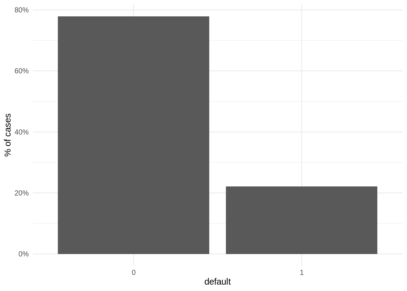
Note that less than 25% of cases are positive. This is a dataset with class imbalance, where the vast majority of observations belong to a category, usually the negative. Datasets with class imbalance are hard to predict, as algorithms can reach high values of accuracy predicting most observations as negative. In problems like loan default of fraud prediction we are interested in detecting all positive cases, as the cost of a false negative is much higher than a false positive. Therefore, sensitivity is more important than global accuracy.
Let’s set the target variable as factor, being the first level the one of the positive class.
LoanDefaults <- LoanDefaults %>%
  mutate(default = factor(default, levels = c("1", "0")))
We use initial_split to generate train and test sets. Here it is important that both sets have the same proportion of positives, so we use strata = "default".
set.seed(1313)
split <- initial_split(LoanDefaults, prop = 0.9, strata = "default")
The preprocessing of features is established with a recipe. The features transformations of this recipe are:
- Removing the
IDvariable. - Create a
payment_statusvariable equal to 0 ifPAY_0is zero or negative and 1 otherwise. - Removing variables
PAY_0toPAY_6. - Transform
SEXinto a factor with descriptive labels. - Setting to
NAvalues ofMARRIAGEandEDUCATIONdo not considered in the dataset description, and transform them into factors with descriptive labels. - Imputing
NAvalues ofMARRIAGEandEDUCATIONusing k nearest neighbors.
recipe <- training(split) %>%
  recipe(default ~ .) %>%
  step_rm(ID) %>%
  step_mutate(payment_status = ifelse(PAY_0 < 1, 0, PAY_0)) %>%
  step_rm(PAY_0:PAY_6) %>%
  step_num2factor(SEX, levels = c("male", "female")) %>%
  step_mutate(MARRIAGE = ifelse(!MARRIAGE %in% 1:3, NA, MARRIAGE)) %>%
  step_mutate(EDUCATION = ifelse(!EDUCATION %in% 1:4, NA, EDUCATION)) %>%
  step_num2factor(MARRIAGE, levels = c("marriage", "single", "others")) %>%
  step_num2factor(EDUCATION, levels = c("graduate", "university", "high_school", "others")) %>%
  step_impute_knn(all_predictors(), neighbors = 3)
Now I can obtain train and test sets using the recipe.
train <- recipe %>% prep() %>% juice()
test <- recipe %>% prep() %>% bake(new_data = testing(split))
Predicting with decision trees
To have a benchmark for random forest performance, I am training a decision tree using rpart with a value small enough of cp.
dt <- rpart(default ~ . , train, cp = 0.001)
rpart.plot(dt)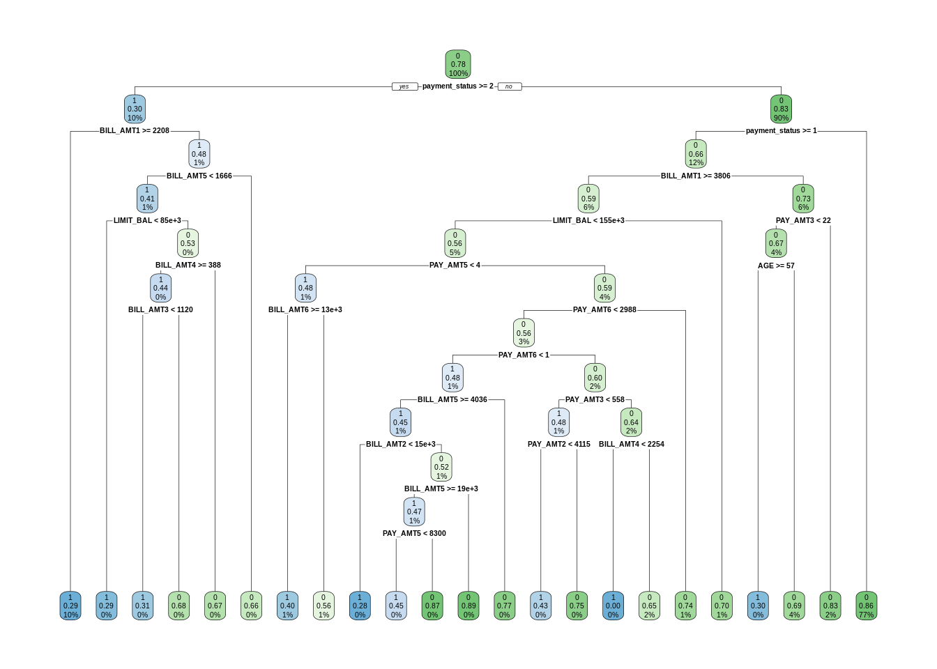
Predicting with random forests
The training of random forests is performed with the ranger function. Its main arguments are:
- a formula specifying the target and predictors.
- the dataset to train the model.
num.trees, the number of trees to train.mtry, the number of variables to possibly split at in each node. I am using the default, equal to the rounded down square root of the number of variables.importance, the variable importance mode.
rf <- ranger(default ~ ., train,
             num.trees = 50,
             importance = "impurity")
Here is some information of the resulting model:
rf## Ranger result
##
## Call:
## ranger(default ~ ., train, num.trees = 50, importance = "impurity")
##
## Type: Classification
## Number of trees: 50
## Sample size: 26999
## Number of independent variables: 18
## Mtry: 4
## Target node size: 1
## Variable importance mode: impurity
## Splitrule: gini
## OOB prediction error: 18.69 %Prediction of train and test sets
Let’s store in a pred_train data frame the actual value of the target variable in the train set, together with the prediction with decision tress dt and the prediction of random forests rf for the train set.
pred_train <- tibble(value = train$default,
                  dt = predict(dt, train, type = "class"),
                  rf =  predict(rf, train)$predictions)
The confusion matrix for decision tree:
pred_train %>%
  conf_mat(truth = value, estimate = dt)
## Truth
## Prediction 1 0
## 1 2248 984
## 0 3724 20043The confusion matrix for the random forest:
pred_train %>%
  conf_mat(truth = value, estimate = rf)
## Truth
## Prediction 1 0
## 1 5818 18
## 0 154 21009Let’s obtain the predictions on the test set…
pred_test <- tibble(value = factor(test$default),
                  dt = predict(dt, test, type = "class"),
                  rf = predict(rf, test)$predictions)
… and examine the confusion matrix.
pred_test %>%
  conf_mat(truth = value, estimate = dt)
## Truth
## Prediction 1 0
## 1 234 131
## 0 430 2206pred_test %>%
conf_mat(truth = value, estimate = rf)## Truth
## Prediction 1 0
## 1 236 119
## 0 428 2218We can see that there is some overfitting to the train set. Let’s compute accuracy, sensitivity and specificity for the two measures and sets. As we obtain a tidy data frame of measures for each combination, we can merge them and present it in a single plot.
m <- metric_set(accuracy, sens, spec)

train_dt <-
  pred_train %>% m(truth = value, estimate = dt) %>%
  mutate(set = "train", method = "dt") %>%
  select(set, method, .metric, .estimate)

test_dt <-
  pred_test %>% m(truth = value, estimate = dt) %>%
  mutate(set = "test", method = "dt") %>%
  select(set, method, .metric, .estimate)

train_rf <-
  pred_train %>% m(truth = value, estimate = rf) %>%
  mutate(set = "train", method = "rf") %>%
  select(set, method, .metric, .estimate)

test_rf <-
  pred_test %>% m(truth = value, estimate = rf) %>%
  mutate(set = "test", method = "rf") %>%
  select(set, method, .metric, .estimate)

bind_rows(train_dt, test_dt, train_rf, test_rf) %>%
  ggplot(aes(.metric, .estimate, fill = set)) +
  geom_col(position = "dodge") +
  facet_grid(. ~ method) +
  scale_fill_manual(name = "set", values = c("#66CC00", "#0066CC")) +
  theme_minimal()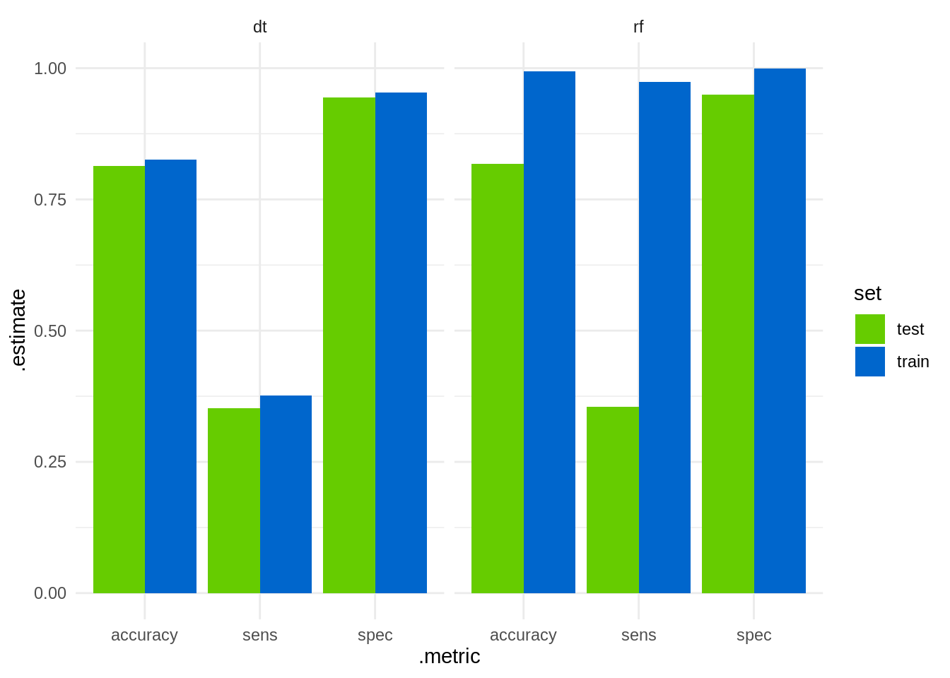
We observe that random forests have high sensitivity (accurate prediction of the positive case), but both methods perform simlilary (and poorly) on the test set.
Variable importance
Being a method based on decision trees, we can obtain values of variabe importance. Here I am obtaining variable importance for decision trees and random forests and presenting them together in a chart. I am using fct_reorder from forcats to arrange variables by order of importance.
vi_dt <- tibble(var = names(dt$variable.importance), vi = dt$variable.importance, t = "dt")
vi_rf <- tibble(var = names(rf$variable.importance), vi = rf$variable.importance, t = "rf")
vi <- bind_rows(vi_dt, vi_rf)
vi <- vi %>% arrange(vi)
vi %>%
  mutate(var = fct_reorder(var, vi)) %>%
ggplot(aes(var, vi, fill = t)) +
  geom_col(position = "dodge") +
  coord_flip() +
  theme_minimal() +
  scale_fill_manual(name = "method", values = c("#CC0000", "#FF8000")) +
  labs(title = "comparing variable importance", x = "variable importance", y = "variable")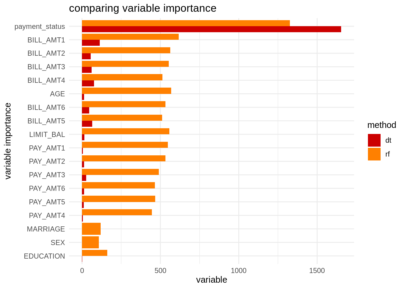
We observe that, while the decision tree is using a subset of the features, random forests is using all variables. The variables not used in the decision tree have low variable importance in the random forest.
How to improve this prediction
Although random forests had better results than the single decision on the train set, this advantage has vanished in the test set. We can undertake two measures to try to improve this result:
- Prediction in datasets with class imbalance can be using balanced train sets. We can achieve this through undersampling (reducing the number of negative cases) or oversampling (adding artificial positive cases).
- Random forests tend to overfit to the train test. We can remedy this doing hyperparameter tuning to both models using cross validation.
References
Kuhn, M. & Vaughan, D. (2022). Random forests via ranger. https://parsnip.tidymodels.org/reference/details_rand_forest_ranger.html
* Wright, M. N. & Ziegler, A. (2017). ranger: a fast implementation of random forests for high dimensional data in C++ and R. Journal of Statistical Software, 77(1). http://dx.doi.org/10.18637/jss.v077.i01
* Wunderbald, B. (2019). Introduction to Random Forests in R. https://brunaw.com/slides/rladies-dublin/RF/intro-to-rf.html#1. Presented in the R Ladies Meetup (Dublin).
## R version 4.2.0 (2022-04-22)
## Platform: x86_64-pc-linux-gnu (64-bit)
## Running under: Linux Mint 19.2
##
## Matrix products: default
## BLAS:   /usr/lib/x86_64-linux-gnu/openblas/libblas.so.3
## LAPACK: /usr/lib/x86_64-linux-gnu/libopenblasp-r0.2.20.so
##
## locale:
##  [1] LC_CTYPE=es_ES.UTF-8       LC_NUMERIC=C
##  [3] LC_TIME=es_ES.UTF-8        LC_COLLATE=es_ES.UTF-8
##  [5] LC_MONETARY=es_ES.UTF-8    LC_MESSAGES=es_ES.UTF-8
##  [7] LC_PAPER=es_ES.UTF-8       LC_NAME=C
##  [9] LC_ADDRESS=C               LC_TELEPHONE=C
## [11] LC_MEASUREMENT=es_ES.UTF-8 LC_IDENTIFICATION=C
##
## attached base packages:
## [1] stats     graphics  grDevices utils     datasets  methods   base
##
## other attached packages:
##  [1] rpart.plot_3.1.0   rpart_4.1.16       BAdatasets_0.1.0   forcats_0.5.1
##  [5] yardstick_0.0.9    workflowsets_0.2.1 workflows_0.2.6    tune_0.2.0
##  [9] tidyr_1.2.0        tibble_3.1.6       rsample_0.1.1      recipes_0.2.0
## [13] purrr_0.3.4        parsnip_0.2.1      modeldata_0.1.1    infer_1.0.0
## [17] ggplot2_3.3.5      dplyr_1.0.9        dials_0.1.1        scales_1.2.0
## [21] broom_0.8.0        tidymodels_0.2.0   ranger_0.13.1
##
## loaded via a namespace (and not attached):
##  [1] lubridate_1.8.0    DiceDesign_1.9     tools_4.2.0        backports_1.4.1
##  [5] bslib_0.3.1        utf8_1.2.2         R6_2.5.1           DBI_1.1.2
##  [9] colorspace_2.0-3   nnet_7.3-17        withr_2.5.0        tidyselect_1.1.2
## [13] compiler_4.2.0     cli_3.3.0          labeling_0.4.2     bookdown_0.26
## [17] sass_0.4.1         stringr_1.4.0      digest_0.6.29      rmarkdown_2.14
## [21] pkgconfig_2.0.3    htmltools_0.5.2    parallelly_1.31.1  lhs_1.1.5
## [25] highr_0.9          fastmap_1.1.0      rlang_1.0.2        rstudioapi_0.13
## [29] farver_2.1.0       jquerylib_0.1.4    generics_0.1.2     jsonlite_1.8.0
## [33] magrittr_2.0.3     Matrix_1.4-1       Rcpp_1.0.8.3       munsell_0.5.0
## [37] fansi_1.0.3        GPfit_1.0-8        lifecycle_1.0.1    furrr_0.3.0
## [41] stringi_1.7.6      pROC_1.18.0        yaml_2.3.5         MASS_7.3-58
## [45] plyr_1.8.7         grid_4.2.0         parallel_4.2.0     listenv_0.8.0
## [49] crayon_1.5.1       lattice_0.20-45    splines_4.2.0      knitr_1.39
## [53] pillar_1.7.0       future.apply_1.9.0 codetools_0.2-18   glue_1.6.2
## [57] evaluate_0.15      blogdown_1.9       vctrs_0.4.1        foreach_1.5.2
## [61] gtable_0.3.0       future_1.25.0      assertthat_0.2.1   xfun_0.30
## [65] gower_1.0.0        prodlim_2019.11.13 class_7.3-20       survival_3.2-13
## [69] timeDate_3043.102  iterators_1.0.14   hardhat_0.2.0      lava_1.6.10
## [73] globals_0.14.0     ellipsis_0.3.2     ipred_0.9-12