Null and alternative hypothesis

Let’s suppose that we want to know if the mean of a population is different from zero. In the null hypothesis, the effect we are looking for does not exists, so the population mean will be zero:

\[H_0 : \mu = 0\]

The alternative hypothesis holds if the null hypothesis does not:

\[H_1 : \mu \neq 0\]

In most cases, the null hypothesis is the absence of effect, while the alternative hypothesis is related with the presence of effect. We can know if the effect exists if we can discard the null hypothesis with a level of significance.

Underlying probability distribution

We don’t really know the population mean \(\mu\), as we would need access to the whole population, something usually impossible or not practical. All we can get is a sample mean \(\bar{x}\) from a sample of \(n\) elements from the population. As we will get a different value of \(\bar{x}\) for each sample, \(\bar{x}\) is a random variable with a probability distribution.

We need to know the distribution of \(\bar{x}\) if the null hypothesis is true. We can use the central limit theorem to know that:

\[ \frac{\bar{x} - \mu}{\sigma/\sqrt{n}} \sim t_{n-1} \]

Where \(t_{n-1}\) is a t-Student distribution with \(n-1\) degrees of freedom, and \(s\) the sample standard deviation. If \(n\) is large enough we can make the approximation:

\[ \frac{\bar{x} - \mu}{s/\sqrt{n}} \sim N\left(0,1\right) \]

The plot below shows the differences between density functions of t-Student of low \(n\) and the \(N\left(0,1\right)\). It shows that it is safe to approximate t-Student to normal distribution for large values of \(n\).

ggplot(data.frame(x = c(-4, 4)), aes(x)) +
  stat_function(fun = dnorm) +
  stat_function(fun = dt, args = list(df=8), color = "red") +
  stat_function(fun = dt, args = list(df=5), color = "blue") +
  annotate(geom = "text", x = 2, y = 0.3, label = "normal N(0,1)", hjust = "left") +
  annotate(geom = "text", x = 2, y = 0.27, label = "t-Student n=8", color = "red", hjust = "left") +
  annotate(geom = "text", x = 2, y = 0.24, label = "t-Student n=5", color = "blue", hjust = "left") +
  theme_bw() +
  labs(title = "t-Student and normal distribution", x = "", y = "")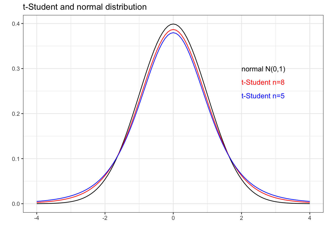

Significance level

To make the hypothesis test from a sample we need to compute the value:

\[\frac{\bar{x} - \mu}{s/\sqrt{n}} \]

What values is likely to take this value if \(H_0\) is true? The plot below presents a \(N\left(0,1\right)\) distribution. The tail values depicted in blue are unlikely to occur in this distribution: in fact each tail has a probability of \(p = 0.025\), so the probability of falling in any of the two tails is \(p = 0.05\).

p <- 0.025
tail_low <- seq(-4, qnorm(p), 0.01)
df_tl <- data.frame(x=c(tail_low,qnorm(p)), y =c(dnorm(tail_low),0))
tail_high <- seq(qnorm(1-p), 4, 0.01)
df_th <- data.frame(x=c(qnorm(1-p),tail_high), y=c(0,dnorm(tail_high)))

ggplot(data.frame(x = c(-4, 4)), aes(x)) +
  stat_function(fun = dnorm) +
  geom_polygon(data = df_tl, aes(x,y), fill = "#99CCFF") +
  geom_polygon(data = df_th, aes(x,y), fill = "#99CCFF") +
  geom_vline(xintercept = qnorm(p), lty = "dashed", lwd = 0.3) +
  geom_vline(xintercept = qnorm(1-p), lty = "dashed", lwd = 0.3) +
  annotate(geom = "text", -1.97, 0.1, label = "-1.96", hjust = "right") +
  annotate(geom = "text", 1.97, 0.1, label = "1.96", hjust = "left") +
  theme_classic() +
  labs(x="", y="")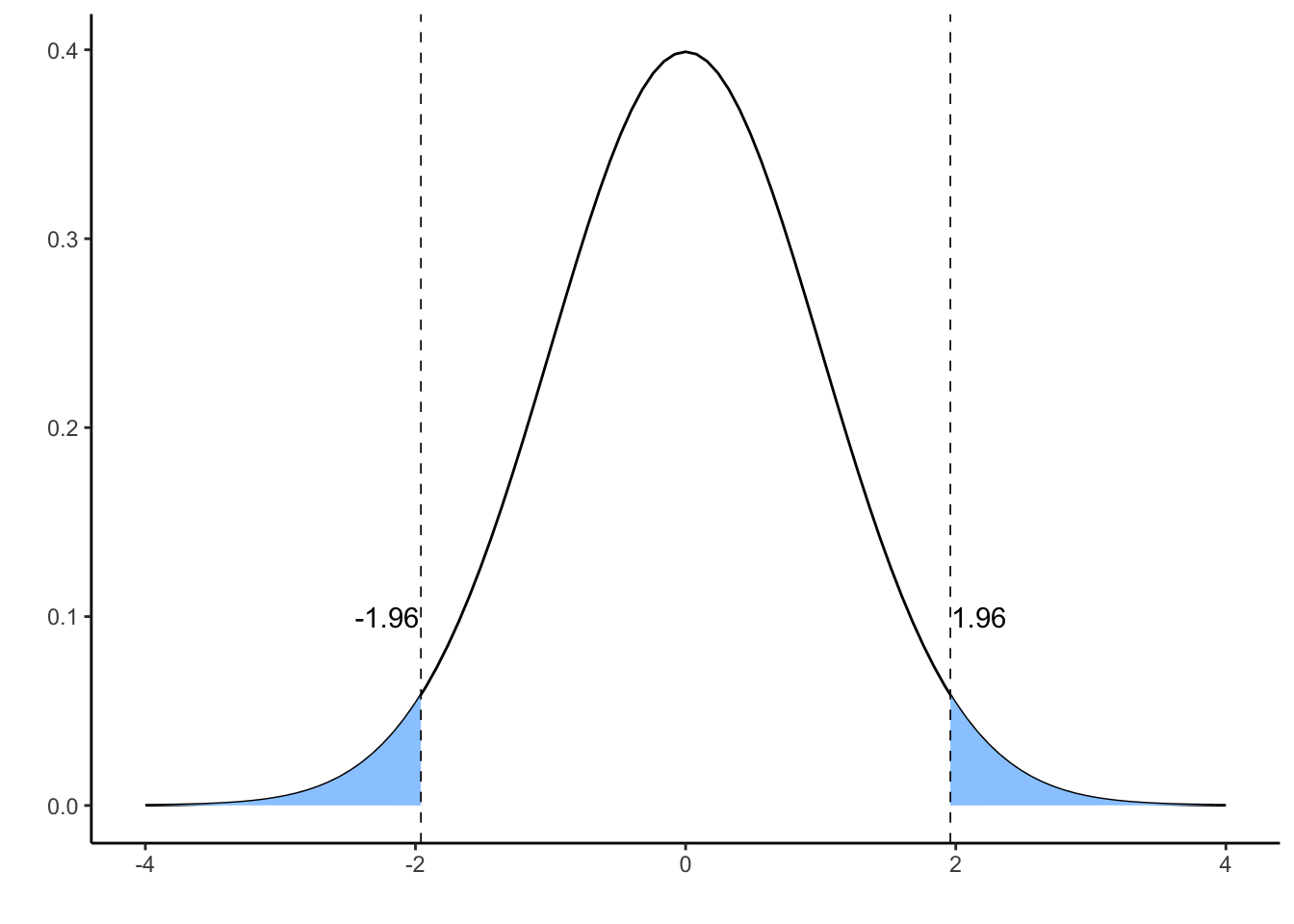

We can obtain the tail values doing:

qnorm(p)

## [1] -1.959964

qnorm(1-p)

## [1] 1.959964

We have two alternative explanations for an observation above 1.96 or below -1.96:

• It is an unfrequent sample from a population for which the null hypothesis is true. Salues outside the interval \(\left[-1.96, 1.96\right]\) can occur with \(p=0.05\).
• The null hypothesis is false.

This is the meaning of the p-value:

The p-value is the probability of observing the obtained value or one more extreme if the hull hypothesis is true.

The threshold for the p-value to reject a null hypothesis is a decision to be taken by the investigator. A common threshold value in many fields is \(p=0.05\), although in some circumstances it is wise to take an even lower value. So, if we observe a p-value below 0.05, we reject the null hypothesis and consider that the alternative hypothesis is true.

Errors when the null hypothesis is true

Let’s see what happens if we perform many tests of hypotheses when the null hypothesis is true. We will use this code to examine that:

set.seed(1313)
p_values_mu0 <- sapply(1:10000, function(x){
  sample <- rnorm(n = 100, mean = 0, sd = 1)
  f <- t.test(sample, mu = 0)
  return(f$p.value)
})

This code obtains 10,000 times a sample of size 100 from a population of a normal distribution with mean zero and standard deviation one. Then, it tests if the population mean is zero using t.test, and stores the p-value obtained from the test. So we have 10,000 different p-values.

Let’s see a representation of the distribution of the obtained p-values:

ggplot(data.frame(p = p_values_mu0), aes(p)) + 
  geom_histogram(binwidth = 0.05, center = 0.025, fill = c("#FF9999", rep("#C0C0C0", 19)), color = "#606060") +
  theme_bw() +
  scale_x_continuous(name="p-value", breaks = seq(0, 1, 0.1))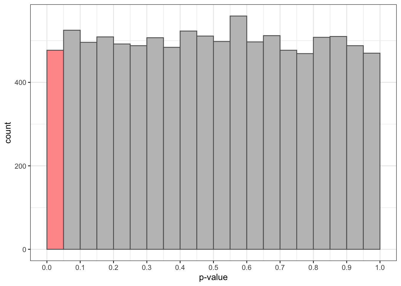

The distribution of p is uniform: if the null hypothesis is true, any p-value has the same probability. The bar in red presents the situations when we refuse the null hypothesis with a significance level of 0.05. In this situations, we are commiting a Type I error.

Errors when the null hypothesis is false

Let’s make a slightly different experiment:

p_values_mu1 <- sapply(1:10000, function(x){
  sample <- rnorm(n = 100, mean = 0.2, sd = 1)
  f <- t.test(sample, mu = 0)
  return(f$p.value)
})

Now the population mean is not zero, so we know that the null hypothesis that the mean is zero is false. Let’s see what p-values we obtain:

ggplot(data.frame(p = p_values_mu1), aes(p)) + 
  geom_histogram(binwidth = 0.05, center = 0.025, fill = c("#C0C0C0", rep("#FF9999", 19)), color = "#606060") +
  theme_bw() +
  scale_x_continuous(name="p-value", breaks = seq(0, 1, 0.1), limits = c(0,1))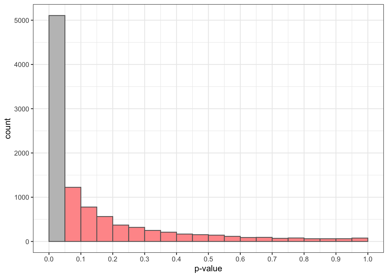

The red bars are of p-values above the significance level of 0.05. There we are accepting the null hypothesis when it is false. This is a Type II error. We observe that the probability of this error is quite high, around 0.5.

We can improve the statistical power of this test increasing the sample size from 100 to 1000:

p_values_mu12 <- sapply(1:10000, function(x){
  sample <- rnorm(n = 1000, mean = 0.2, sd = 1)
  f <- t.test(sample, mu = 0)
  return(f$p.value)
})

Now that sample size is 1000, the probability of Type II error has lowered to near zero:

ggplot(data.frame(p = p_values_mu12), aes(p)) + 
  geom_histogram(binwidth = 0.05, center = 0.025, fill = c("#C0C0C0", rep("#FF9999", 19)), color = "#606060") +
  theme_bw() +
  scale_x_continuous(name="p value", breaks = seq(0, 1, 0.1), limits = c(0,1))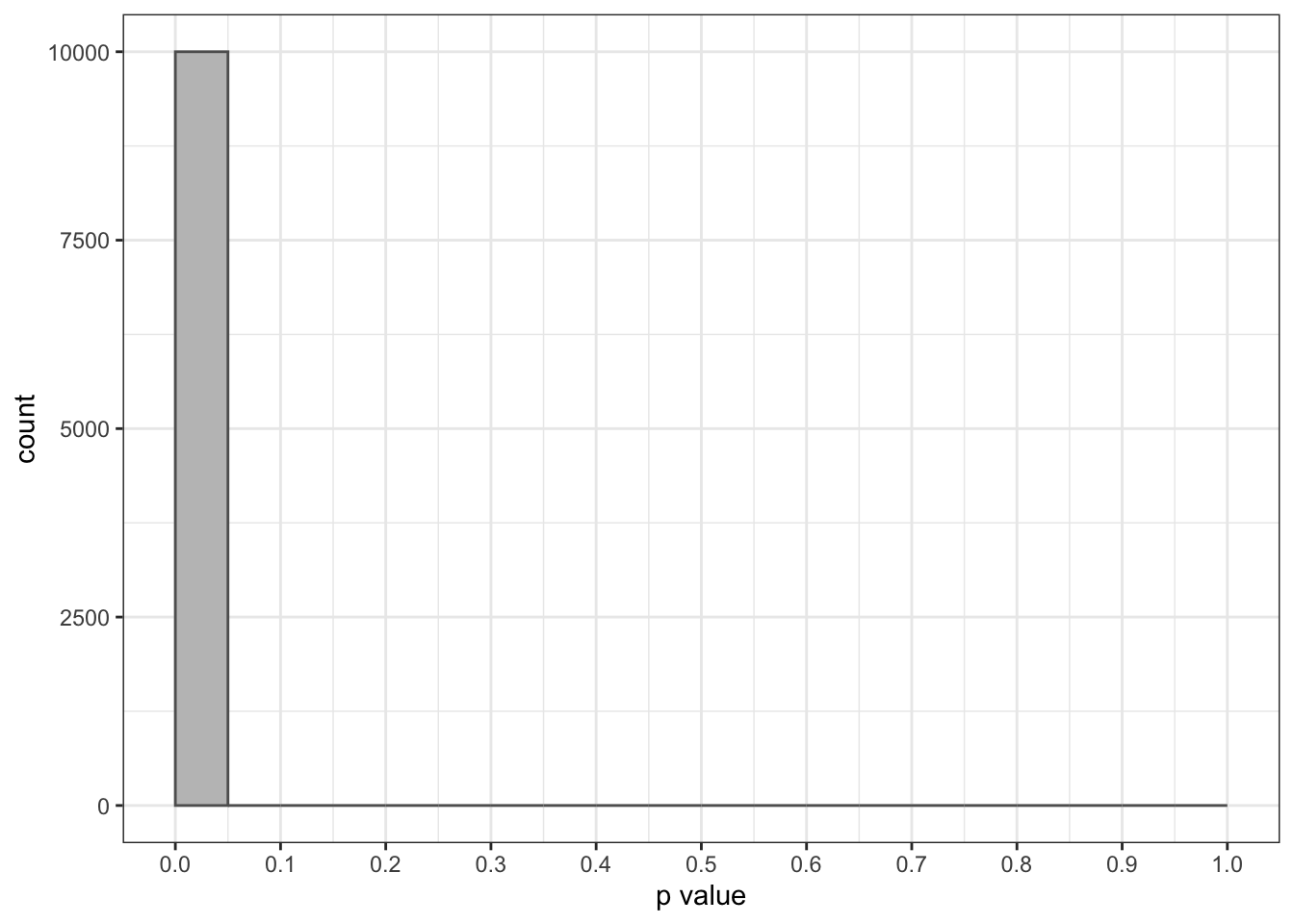

It is important to keep in mind is that when we do not reject the null hypothesis, we cannot be sure whether it is true or not. It can be either that the null hypothesis is true and there is no effect, or that the effect is too small to be observed with the statistical power of our sample.

Type I and type II errors in hypothesis testing

Hypothesis testing is an important tool in quantitative scientific research. A bad use of hypothesis testing, together with the incentives of the research job market, is in the core of the reproductibility crisis of scientific research based on statistical inference. It is of great importance that any scientist understands hypothesis testing correctly.

There are two different types of error in hypothesis testing:

• We commit a Type I error when we reject the null hypothesis when it is true. This means that we are detecting an effect when it is not present.
• We commit a Type II error when we do not reject the null hypothesis when it is false. This means that we are not detecting an effect when it is present. We can reduce the probability of Type II error increasing the statistical power of the experiment, which usually means increasing the sample size.

Further reading

• Annotations in ggplot: https://ggplot2-book.org/annotations.html
• Misuse of p-values: https://en.wikipedia.org/wiki/Misuse_of_p-values

Built with R 4.1.0 and ggplot2 3.3.4