Calculating Confidence Intervals

Let’s start obtainining a sample of a normal distribution with mean zero and standard deviation one with the rnorm() function. If I want a sample of 100 observations we proceed as follows:

set.seed(1212)
x <- rnorm(100)

Let’s use t.test() to check if the population mean is zero:

t.test(x)

## 
## 	One Sample t-test
## 
## data:  x
## t = -0.84443, df = 99, p-value = 0.4005
## alternative hypothesis: true mean is not equal to 0
## 95 percent confidence interval:
##  -0.2835738  0.1142651
## sample estimates:
##   mean of x 
## -0.08465435

We observe that:

• The p-value of the hypothesis testing is higher than the standard threshold of 0.05.
• The confidence interval contains the hypothesized population mean of zero.

Therefore, we cannot reject the null hypothesis that the mean is equal to zero.

What would happen if we perform this tests to many samples from the same distribution? If we want to store them in a data frame, we might want to use broom::tidy() to obtain the result in a tibble format:

tidy(t.test(x))

## # A tibble: 1 × 8
##   estimate statistic p.value parameter conf.low conf.high method     alternative
##      <dbl>     <dbl>   <dbl>     <dbl>    <dbl>     <dbl> <chr>      <chr>      
## 1  -0.0847    -0.844   0.400        99   -0.284     0.114 One Sampl… two.sided

Let’s wrap it together in a conf_int() function that takes the sample size n as input and:

• generates a sample from a normal distribution with rnorm().
• performs the t.test() of the sample mean.
• stores the output in tidy format, retaining the variables of interest: the mean estimate, the lower and upper bound of the confidence interval conf.low and conf.high and the p.value.

conf_int <- function(n = 100, mean = 0, sd = 1){
  sample <- rnorm(n = n, mean = mean, sd = sd)
  test <- t.test(sample)
  result <- tidy(test) |>
    select(estimate, conf.low, conf.high, p.value)
  return(result)
}

A run of the function leads to:

set.seed(1212)
conf_int()

## # A tibble: 1 × 4
##   estimate conf.low conf.high p.value
##      <dbl>    <dbl>     <dbl>   <dbl>
## 1  -0.0847   -0.284     0.114   0.400

Now we can use purrr::map_dfr() to wrap the results of many runs of conf_int() in a single tibble. Once obtained, we can check whether zero is within the confidence interval and store the result in a column, and give and id to each observation. All of this is done in the set_intervals() function, that takes as arguments n and the number of samples sample.

set_intervals <- function(sample  = 100, n = 100, mean = 0, sd = 1){
  
  intervals <- map_dfr(1:sample, ~ conf_int(n = n, mean = mean, sd = sd))
  
  intervals <- intervals |>
    mutate(id = 1:n(),
           result = ifelse(sign(conf.low) == sign(conf.high), "accept", "reject")) |>
    relocate(id)
  
  return(intervals)
}

The outcome of the function looks like:

set.seed(1111)
intervals <- set_intervals()
intervals

## # A tibble: 100 × 6
##       id estimate conf.low conf.high p.value result
##    <int>    <dbl>    <dbl>     <dbl>   <dbl> <chr> 
##  1     1   0.242   0.0225    0.461   0.0310  accept
##  2     2   0.210  -0.00567   0.425   0.0562  reject
##  3     3  -0.0705 -0.250     0.109   0.438   reject
##  4     4  -0.0869 -0.269     0.0952  0.346   reject
##  5     5  -0.0155 -0.215     0.184   0.878   reject
##  6     6  -0.190  -0.373    -0.00657 0.0425  accept
##  7     7  -0.0926 -0.290     0.105   0.354   reject
##  8     8  -0.281  -0.478    -0.0847  0.00549 accept
##  9     9  -0.0622 -0.262     0.138   0.539   reject
## 10    10   0.0850 -0.0901    0.260   0.338   reject
## # ℹ 90 more rows

Plotting many Confidence Intervals

Let’s plot the results, using geom_point() for the sample mean and geom_segment():

intervals |>
  ggplot(aes(estimate, id, color = result)) +
  geom_point() +
  geom_segment(aes(x = conf.low, y = id, xend = conf.high, yend = id, color = result))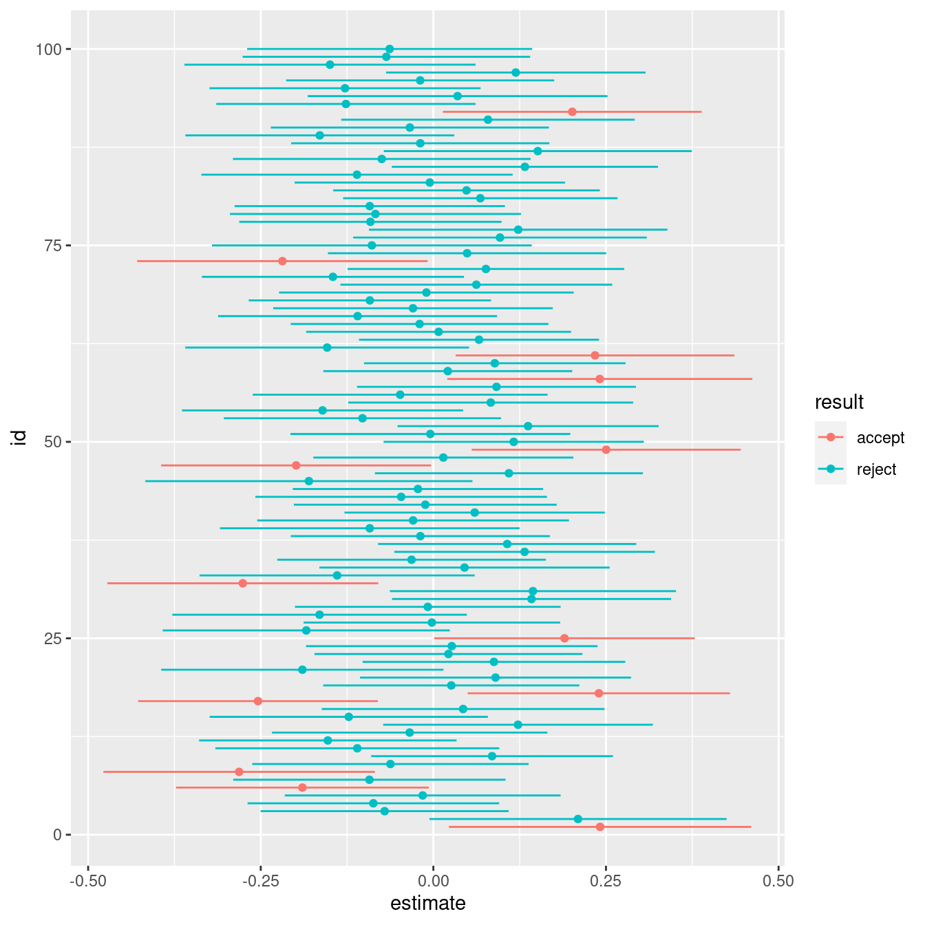

A nicer version of the same plot:

intervals |>
  ggplot(aes(estimate, id, color = result)) +
  geom_point() +
  geom_segment(aes(x = conf.low, y = id, xend = conf.high, yend = id, color = result)) +
  geom_vline(xintercept = 0, linetype = "dashed") +
  ggtitle("Several confidence intervals") +
  scale_color_manual(values = c("#FF3333", "#009900")) +
  theme_minimal() +
  theme(axis.text.y = element_blank(), 
        axis.title.y = element_blank(),
        axis.title.x = element_blank(),
        legend.position = "none",
        plot.title.position = "plot")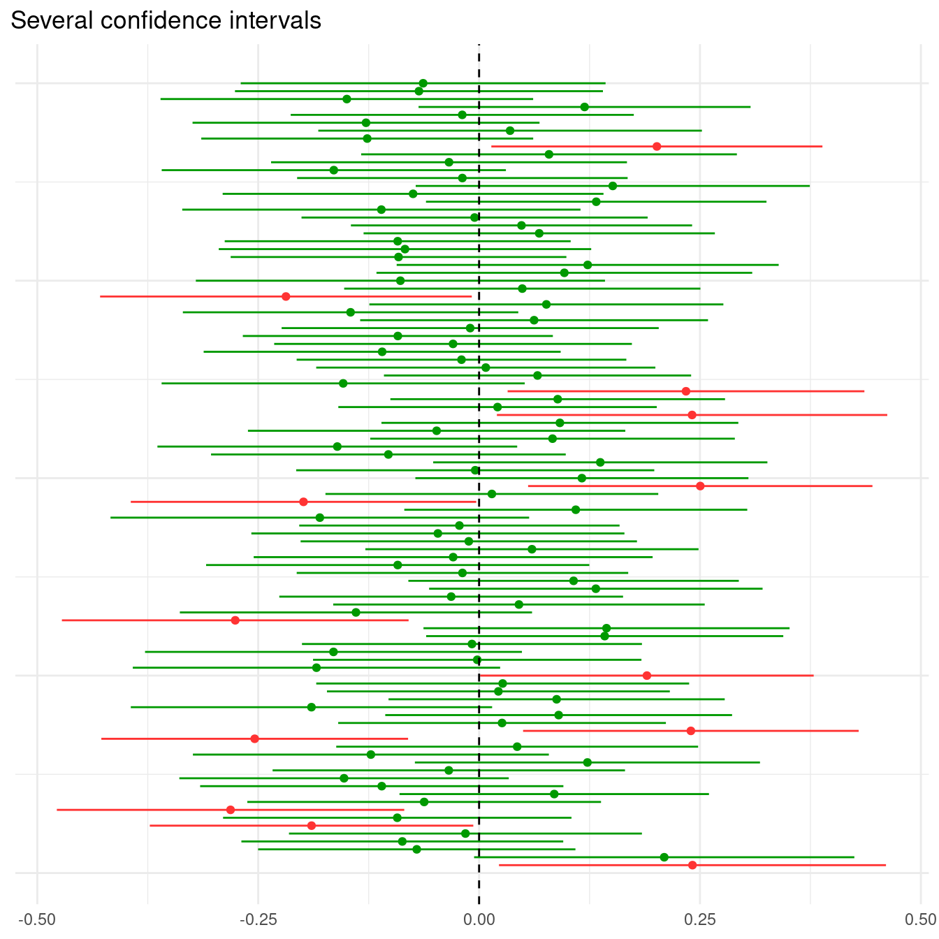

In this case, the population that we are taking the samples from has a mean equal to zero, so that the null hypothesis that the population mean is equal is zero is true. Therefore, we observe that most of the confidence intervals contain the zero (in green), but some of them do not (in red).

intervals |>
  group_by(result) |>
  count()

## # A tibble: 2 × 2
## # Groups:   result [2]
##   result     n
##   <chr>  <int>
## 1 accept    13
## 2 reject    87

Specifically, in 13 out of the 100 intervals, we have rejected the null hypothesis, comiting a Type I error. Let’s relate this with p-values evaluating the minimum and maximum values for the two values of result:

intervals |>
  group_by(result) |>
  summarise(min_pvalue = min(p.value), max_pvalue = max(p.value))

## # A tibble: 2 × 3
##   result min_pvalue max_pvalue
##   <chr>       <dbl>      <dbl>
## 1 accept    0.00456     0.0486
## 2 reject    0.0562      0.982

In all cases that the confidence interval does not include zero, the p-value is smaller than 0.05. We observe, though, that this is happening 13% of the time, more than the expected 5%. Let’s pick a set of 1,000 samples to get a more precise estimation of probability.

set.seed(3333)
intervals_large <- set_intervals(sample = 1000)

Let’s see in how many samples of intervals_large we are committing a Type I error:

intervals_large |>
  group_by(result) |>
  count()

## # A tibble: 2 × 2
## # Groups:   result [2]
##   result     n
##   <chr>  <int>
## 1 accept    48
## 2 reject   952

Now the number of Type I errors is closer to 5%.

Confidence Intervals and Variance

The variability on the original sample affects the confidence interval: the smaller the variance of the same, the smaller the width of the interval. To illustrate this, let’s build a set of intervals taken from a population of smaller variance and compare the results with the previous plot.

set.seed(5555)
intervals_sv <- set_intervals(sd = 0.5)

two_intervals <- bind_rows(intervals |> mutate(sd = 1),
                           intervals_sv |> mutate(sd = 0.5))

two_intervals |>
  ggplot(aes(estimate, id, color = result)) +
  geom_point() +
  geom_segment(aes(x = conf.low, y = id, xend = conf.high, yend = id, color = result)) +
  facet_grid(. ~ sd, labeller = label_both) +
  geom_vline(xintercept = 0, linetype = "dashed") +
  ggtitle("Effect of sd on confidence intervals") +
  scale_color_manual(values = c("#FF3333", "#009900")) +
  theme_minimal() +
  theme(axis.text.y = element_blank(),
        axis.text.x = element_text(size = 6, angle = 90),
        axis.title.y = element_blank(),
        axis.title.x = element_blank(),
        legend.position = "none",
        plot.title.position = "plot",
        strip.text.x = element_text(size = 10),
        strip.background.x = element_rect(fill = "#FFB266", color = "#808080"))

Interpreting Confidence Intervals

In frequentist statistics, a confidence interval is a random interval that contains the (true) population parameter with a probability \(1 - \alpha\). The value \(1 - \alpha\) is the confidence level of the interval.

We can use confidence intervals for hypothesis testing: if the interval does not contain the population parameter defined in the null hypothesis, we can reject the null hypothesis with a probability of Type I error of \(\alpha\). The confidence interval is related with the p-value: if the confidence interval does not contain the expected population parameter, the p-value will be smaller than \(\alpha\).

Session Info

## R version 4.3.3 (2024-02-29)
## Platform: x86_64-pc-linux-gnu (64-bit)
## Running under: Linux Mint 21.1
## 
## Matrix products: default
## BLAS:   /usr/lib/x86_64-linux-gnu/blas/libblas.so.3.10.0 
## LAPACK: /usr/lib/x86_64-linux-gnu/lapack/liblapack.so.3.10.0
## 
## locale:
##  [1] LC_CTYPE=es_ES.UTF-8       LC_NUMERIC=C              
##  [3] LC_TIME=es_ES.UTF-8        LC_COLLATE=es_ES.UTF-8    
##  [5] LC_MONETARY=es_ES.UTF-8    LC_MESSAGES=es_ES.UTF-8   
##  [7] LC_PAPER=es_ES.UTF-8       LC_NAME=C                 
##  [9] LC_ADDRESS=C               LC_TELEPHONE=C            
## [11] LC_MEASUREMENT=es_ES.UTF-8 LC_IDENTIFICATION=C       
## 
## time zone: Europe/Madrid
## tzcode source: system (glibc)
## 
## attached base packages:
## [1] stats     graphics  grDevices utils     datasets  methods   base     
## 
## other attached packages:
##  [1] broom_1.0.5     lubridate_1.9.3 forcats_1.0.0   stringr_1.5.1  
##  [5] dplyr_1.1.4     purrr_1.0.2     readr_2.1.5     tidyr_1.3.0    
##  [9] tibble_3.2.1    ggplot2_3.4.4   tidyverse_2.0.0
## 
## loaded via a namespace (and not attached):
##  [1] sass_0.4.5        utf8_1.2.3        generics_0.1.3    blogdown_1.16    
##  [5] stringi_1.7.12    hms_1.1.3         digest_0.6.31     magrittr_2.0.3   
##  [9] evaluate_0.20     grid_4.3.3        timechange_0.2.0  bookdown_0.33    
## [13] fastmap_1.1.1     jsonlite_1.8.8    backports_1.4.1   fansi_1.0.4      
## [17] scales_1.2.1      jquerylib_0.1.4   cli_3.6.1         rlang_1.1.3      
## [21] munsell_0.5.0     withr_2.5.0       cachem_1.0.7      yaml_2.3.7       
## [25] tools_4.3.3       tzdb_0.3.0        colorspace_2.1-0  vctrs_0.6.4      
## [29] R6_2.5.1          lifecycle_1.0.3   pkgconfig_2.0.3   pillar_1.9.0     
## [33] bslib_0.6.1       gtable_0.3.3      glue_1.6.2        highr_0.10       
## [37] xfun_0.39         tidyselect_1.2.0  rstudioapi_0.15.0 knitr_1.42       
## [41] farver_2.1.1      htmltools_0.5.7   rmarkdown_2.21    labeling_0.4.2   
## [45] compiler_4.3.3