library(tidyverse)
library(broom)
When we are fitting a statistical model, we can be interested in finding what is the influence of an observation on the model. An observation with high influence will affect substantially the value of the parameter estimates.
Let’s examine the influence of observations in the context of linear regression of an dependent variable \(y\) on a set of dependent variables \(x_1, \dots, x_p\):
\[ y_i = \beta_0 + \beta_1x_{i1} + \dots + \beta_px_{ip} + \varepsilon_i \]
We cannot know the population parameters of the above formula, but its estimators:
\[ y_i = b_0 + b_1x_{i1} + \dots + b_px_{ip} + e_i = \hat{y}_i + e_i \]
One can think that all outliers (observations with abnormal values) will be influent observations. But in linear regression, it is frequent that only outliers with high leverage have large influence on parameter estimates. Leverage is a measure of how far away the independent variable values of an observation are from those of the other observations.
Let’s see an example of univariate regression (a single dependent variable x) to clarify these concepts. The red points are 100 normal observations, while observations A to D are added to exemplify leverage and influence.
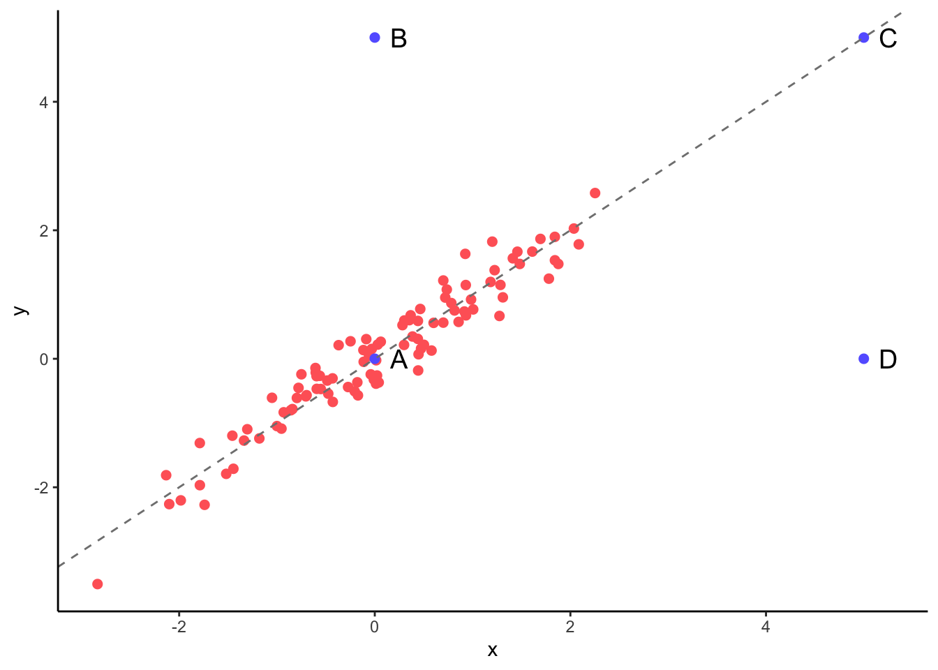
Examining the plot, we see that:
- Observation A is not an outlier, points B, C and D are.
- Observation B is a low-leverage, low-influence point.
- Observation C is a high-leverage, low-influence point.
- Observation D is a high-leverage, high-influence point.
Evaluating influence and leverage
With larger multivariate samples, we need numerical parameters to estinate influence and leverage. Cook’s distance is a measure of influence that compares fitted values \(\hat{y}_j\) with fitted values obtained when observation \(i\) is retrieved from the sample \(\hat{y} _{j \left( i \right)}\):
\[ D_i = \frac{\sum_{j=1}^n \left( \hat{y}_j - \hat{y} _{j \left( i \right)}\right)^2}{p s^2} \]
where \(s^2\) is the observed variance of the residuals.
The leverage of an observation is obtained from the diagonal elements of the hat matrix, that relates fitted values with observed values. In vectorial notation:
\[ \mathbf{\hat{y}} = \mathbf{X} \left( \mathbf{X}^T\mathbf{X} \right)^{-1} \mathbf{X}^T \mathbf{y}= \mathbf{H} \mathbf{y} \]
where \(\mathbf{X}\) is the design matrix, whose rows correspond to observations and columns to independent variables. The elements of the first column of \(\mathbf{X}\) are associated with the intercept and are all equal to one.
The leverage of an observation \(i\) is equal to:
\[ h_{ii} = \frac{\partial \hat{y}_i}{\partial{y_i}} \]
Observations with high leverage will have values of independent variables far from the other variables. This is the case of observations C and D of the above figure.
Cook’s distance and leverage are related through the expression:
\[ D_i = \frac{e_i^2}{ps^2} \left[ \frac{h_{ii}}{\left( 1- h_{ii} \right)^2} \right] \]
From this expression we learn that an influential observation must have a high leverage and a high value of residual. In the above plot, observation D is the one with high values of residuals and leverage.
Examining influence and leverage
Let’s see how can we obtain Cook’s distance and leverage with the broom package. First we obtain the ordinary least squares estimators of the linear regression model doing:
mod <- lm(y ~ x, data)The augment function of broom provides additional information for each observation:
- variable
.hatis equal to leverage. - variable
.cooksdis equal to Cook’s distance.
augment(mod)## # A tibble: 104 x 8
## y x .fitted .resid .hat .sigma .cooksd .std.resid
## <dbl> <dbl> <dbl> <dbl> <dbl> <dbl> <dbl> <dbl>
## 1 -0.242 -0.750 -0.582 0.341 0.0148 0.734 0.00166 0.470
## 2 0.306 -0.0872 -0.0303 0.336 0.0100 0.734 0.00108 0.462
## 3 1.82 1.20 1.04 0.781 0.0163 0.730 0.00962 1.08
## 4 -0.570 -0.172 -0.101 -0.469 0.0103 0.733 0.00217 -0.645
## 5 -0.260 0.0230 0.0614 -0.322 0.00974 0.734 0.000962 -0.442
## 6 1.15 1.28 1.11 0.0381 0.0174 0.734 0.0000245 0.0526
## 7 0.953 0.721 0.642 0.311 0.0115 0.734 0.00107 0.428
## 8 0.272 -0.248 -0.164 0.436 0.0107 0.733 0.00194 0.600
## 9 -0.323 -0.00997 0.0339 -0.357 0.00981 0.733 0.00119 -0.491
## 10 0.752 0.816 0.721 0.0311 0.0122 0.734 0.0000113 0.0428
## # … with 94 more rowsWe can plot those variables in a leverage versus influence plot:
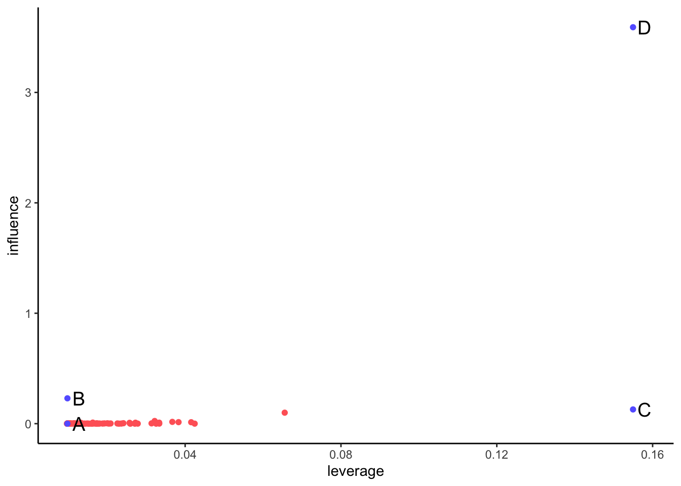
We observe that point D is the only influential observation, with a high value of Cook’s distance. For large samples, observations with \(D_i > 1\) can be considered highly influential.
Examining influence and leverage with the olsrr package
The olsrr package provides a set of tools to build and examine ordinary least squares regression models. Let’s examine how to obtain measures of influence using olsrr.
library(olsrr)The functions ols_plot_cooksd_bar and ols_plot_cooksd_chart allows examining Cook’s distances:
ols_plot_cooksd_chart(mod)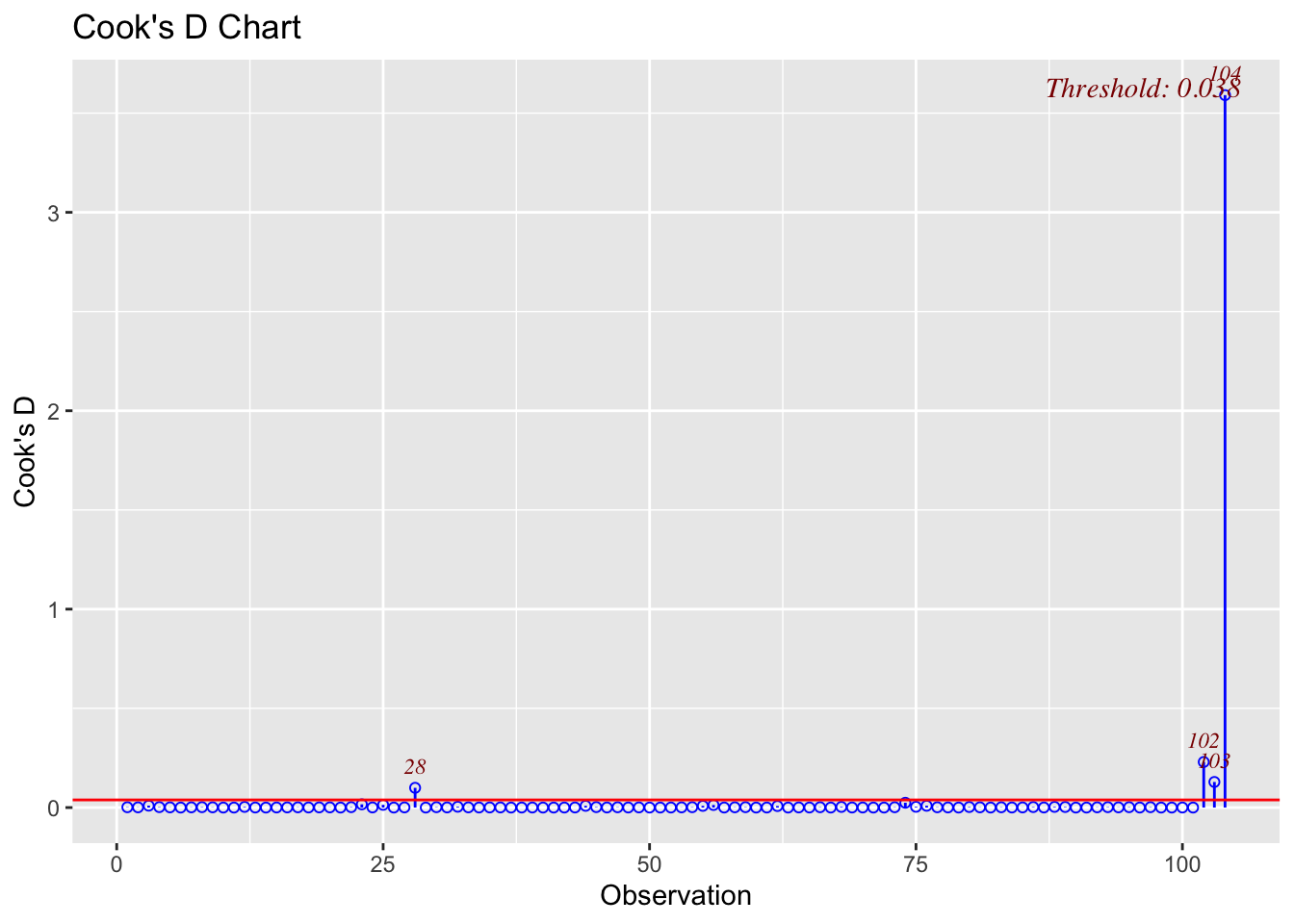
The function ols_plot_dfbetas allows examining how the removal of each observation affects parameter estimates
ols_plot_dfbetas(mod)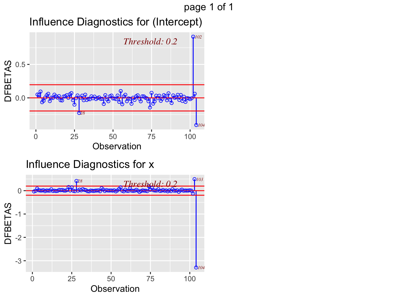
From these plots, we learn that observation B (labelled here as 102) is the one affecting the intercept the most, while observation D or 104 is the one with more influence on the relationship between variables \(y\) and \(x\).
Leverage and influence
In linear regression, the leverage of an observation measures how fare are its values of the independent variables from the rest of observations, while influence measures how much affects the observation to parameter estimates. Cook’s distance is the most used measure of influence. To be influential, an observation must have large values of leverage and residual. We can obtain values of leverage and Cook’s distance from the augment function of the broom package.
Built with R 4.0.3, tidyverse 1.3.0, broom 0.7.5 and olsrr 0.5.3