Implementation of DBSCAN Clustering in R

Jose M Sallan 2025-12-24 9 min read

clustering

Cluster analysis, or clustering, consists of partitioning a set of objects into groups such that objects within the same group (called a cluster) exhibit greater similarity to one another (in some specific sense defined by the analyst) than to those in other clusters.

In this post, I will introduce a clustering technique called discrete-based spatial clustering and applications with noise (DBSCAN) introduced in Ester et al. (1996). In R, this technique is implemented with the dbscan package. In this post I will introduce DBSCAN, its specific approach to clustering and how to perform DBSCAN clustering in R.

library(tidyverse)
library(broom)
library(dbscan)
library(patchwork)

There are two traditional types of clustering algorithms: partitioning and hierarchical algorithms. Partitioning algorithms obtain a partition of the dataset into k clusters, so that the within-clusters square distances are smaller than between-clusters. The best known of these algorithms is k-means. These algorithms generate clusters that tend to be spherical and compact around a cluster center. Hierarchical algorithms create a hierarchical decomposition of the dataset, graphically represented with a dendogram. These techniques are implemented in R base with functions like kmeans() and hclust().

These algorithms are not effective to identify clusters defined as subsets of elements with a higher density within the cluster than outside the cluster and with irregular shapes. Two examples are the two_moons and target datasets, obtained with functions of the fdm2id package.

set.seed(1111)
two_moons <- fdm2id::data.twomoons(sigma = 0.1, graph = FALSE)
target <- fdm2id::data.target2(initn = 600, graph = FALSE)

These datasets have two distinct clusters of irregular shape. Let’s try to detect them using kmeans(). I am using broom::augment() to add the .cluster column to the original dataset.

set.seed(1111)
two_moons_km <- kmeans(two_moons[, 1:2], centers = 2)
target_km <- kmeans(target[, 1:2], centers = 2)

two_moons_km_table <- augment(two_moons_km, data = two_moons)
target_km_table <- augment(target_km, data = target)

Let’s see how kmeans() is performing:

p1 <- ggplot(two_moons_km_table, aes(X, Y, color = .cluster)) +
  geom_point() +
  labs(title = "Two Moons (k-means)", x = NULL, y = NULL) +
  theme_minimal(base_size = 12) +
  theme(legend.position = "bottom")

p2 <- ggplot(target_km_table, aes(X, Y, color = .cluster)) +
  geom_point() +
  labs(title = "Target (k-means)", x = NULL, y = NULL) +
  theme_minimal(base_size = 12) +
  theme(legend.position = "bottom")

p1 + p2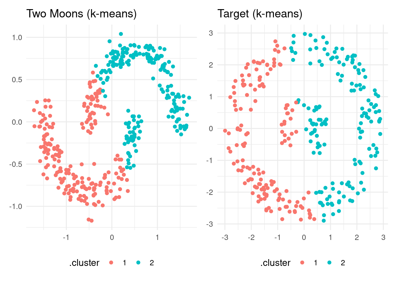

As we can see, k-means is performing poorly on these datasets.

The DBSCAN Algorithm

The DBSCAN algorithm takes a density-based approach to clustering. The algorithm is based on two parameters:

The maximum distance between cluster points. It is the eps argument of the dbscan() function.
The minimum number of points close to a core point of the cluster. It is the minPts argument of the dbscan() function.

Taking this into account, we can make the following definitions:

An element \(p\) of the dataset is a core point if there are at least minPts elements within a distance equal or smaller than eps from it.
An element \(q\) is directly reachable from \(p\) if it is within a distance equal or smaller than eps from \(p\).
\(q\) is density-reachable from \(p\) if there is a path starting at \(p\) and ending at \(q\) where each element \(p_{i+1}\) is directly reachable from \(p_i\). All points of the path must be core points with the probable exception of \(q\).
Two points \(p\) and \(q\) are density-connected if there is a point \(o\) such that \(p\) and \(q\) are reachable from \(o\).
A point is a noise point if it is not reachable from any other points. These points are not assigned to any cluster by the algorithm.

DBSCAN clusters are formed as sets of density-connected points. The points of a cluster that are not core points are border points.

Regarding parameter estimates, minPts is usually set as the dimensions of the dataset plus one. For minPts = 2, the result is similar to a hierachical clustering with the dendogram cut at height eps.

DBSCAN has some relevant differences from other clustering methods:

The number of clusters is not fixed beforehand. Typically small values of eps lead to many small clusters, and large values of eps lead to few large clusters.
There may be noise points that do not belong to any cluster.

As the connectivity between points is based on paths of connected core points rather than the distance from a center point, this algorithm can be adequate to detect clusters of irregular shapes of spatial datasets.

A Small Example

Let’s start with a small example consisting of a two dimensional dataset of twenty points.

x <- c(4, 6, 5, 5, 5, 6, 7, 2, 11, 12, 13, 12, 12, 13, 14, 12, 10, 15, 4, 13)
y <- c(6, 6, 7, 5, 4, 4, 4, 6, 10, 11, 10, 9, 8, 8, 8, 6, 8, 10, 13, 3)

points <- tibble(point = 1:20, x = x, y = y)

ggplot(points, aes(x, y, label = point)) +
  geom_label() +
  theme_minimal() +
  scale_x_continuous(breaks = 1:20) +
  scale_y_continuous(breaks = 1:20)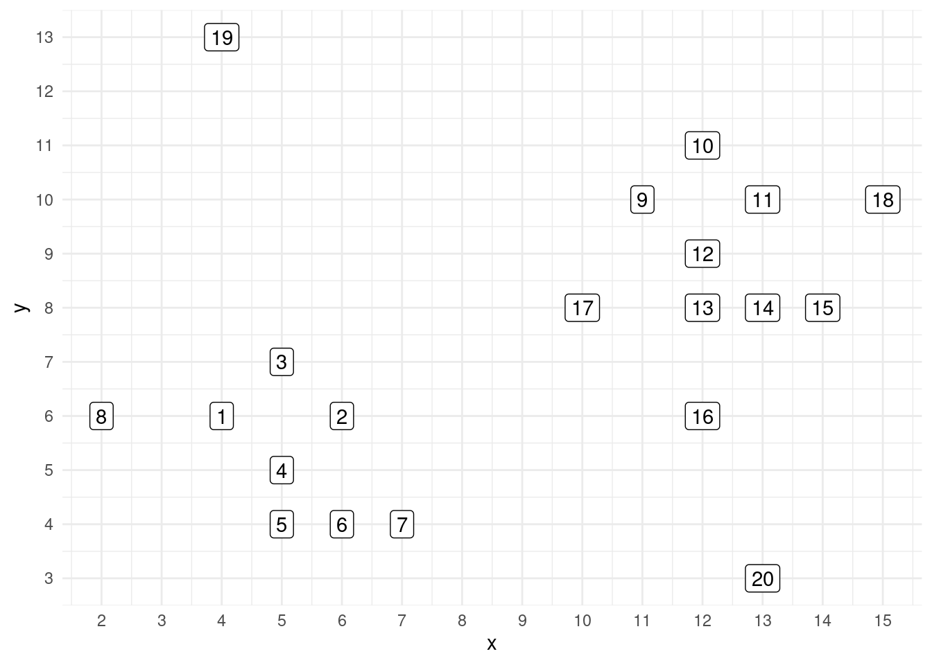

By ocular inspection, we can see two clusters: one of points 1 to 8, and other with points 9 to 18. Points 19 and 20 can be considered noise points.

Let’s consider for this example eps = 3 and minPts = 3. The m_points table includes all pairs of elements with a distance equal or smaller than three.

m_points <- dist(points[, 2:3]) |>
  as.matrix() |>
  as.data.frame() |>
  mutate(row = 1:n()) |>
  pivot_longer(-row, names_to = "col", values_to = "dist") |>
  mutate(col = as.numeric(col)) |>
  filter(row != col)

With this table, we can detect the core points as those with at least minPts elements at a distance equal or smaller than eps.

eps <- 3
minPts <- 3

core <- m_points |>
  filter(dist <= eps) |>
  group_by(row) |>
  summarise(n = n(), .groups = "drop") |>
  filter(n >= minPts) |>
  pull(row)

core

##  [1]  1  2  3  4  5  6  7  9 10 11 12 13 14 15 16 17 18

The core elements are points 1 to 18 except point 8. Let’s identify the border points, that is, density reachable points that are not core points.

reached <- m_points |>
  filter(dist <= eps) |>
  filter(row %in% core) |>
  pull(col) |>
  unique()

reachable <- reached[!reached %in% core]
reachable

## [1] 8

The only border point for this dataset is 8. Let’s see from where it is reached:

m_points |>
  filter(row == 8, dist <= eps)

## # A tibble: 1 × 3
##     row   col  dist
##   <int> <dbl> <dbl>
## 1     8     1     2

Element 8 is only reached by element 1, so it is not a core element. Let’s see another possible peripheral element like 18:

m_points |>
  filter(row == 18, dist <= eps)

## # A tibble: 3 × 3
##     row   col  dist
##   <int> <dbl> <dbl>
## 1    18    11  2   
## 2    18    14  2.83
## 3    18    15  2.24

As 18 has three elements with a distance equal or smaller than eps, it is a core element.

The rest of elements are the noise points:

labels <- 1:20
noise <- labels[!labels %in% c(core, reachable)]
noise

## [1] 19 20

The DBSCAN clustering of this dataset would be:

example_db <- dbscan(points[, 2:3], eps = 3, minPts = 3)
example_db$cluster

##  [1] 1 1 1 1 1 1 1 1 2 2 2 2 2 2 2 2 2 2 0 0

Here is a representation of the clustering, indicating core, border and noise points.

type <- character(20)
type[core[1:7]] <- "c1_core"
type[core[8:17]] <- "c2_core"
type[reachable] <- "c1_border"
type[noise] <- "noise"

points <- points |>
  mutate(type = type)

ggplot(points, aes(x, y, label = point, fill = type)) +
  geom_label(alpha = 0.5) +
  theme_minimal(base_size = 12) +
  scale_x_continuous(breaks = 1:20, name = NULL) +
  scale_y_continuous(breaks = 1:20, name = NULL) +
  scale_fill_manual(values = c("#FF3333", "#FF9933", "#3399FF", "#A0A0A0")) +
  theme(legend.position = "bottom")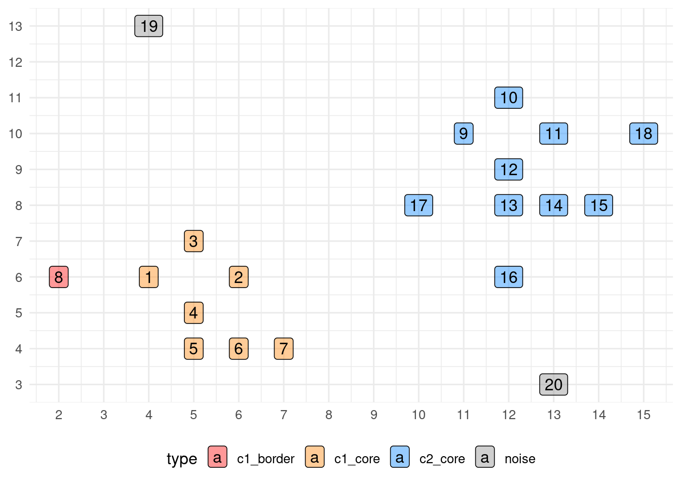

Testing DBSCAN on Spatial Datasets

Let’s see how DBSCAN works in the two_moons and target datasets. I have set minPts = 3 and found eps by trial and error. I have used broom::augment() to add the .cluster column.

set.seed(1111)
two_moons_db <- dbscan(two_moons[, 1:2], eps = 0.25, minPts = 3)
target_db <- dbscan(target[, 1:2], eps = 0.5, minPts = 3)

two_moons_db_table <- augment(two_moons_db, data = two_moons)
target_db_table <- augment(target_db, data = target)

Here is the graphical result:

p1 <- ggplot(two_moons_db_table, aes(X, Y, color = .cluster)) +
  geom_point() +
  labs(title = "Two Moons (DBSCAN)", x = NULL, y = NULL) +
  theme_minimal(base_size = 12) +
  theme(legend.position = "bottom")

p2 <- ggplot(target_db_table, aes(X, Y, color = .cluster)) +
  geom_point() +
  labs(title = "Target (DBSCAN)", x = NULL, y = NULL) +
  theme_minimal(base_size = 12) +
  theme(legend.position = "bottom")

p1 + p2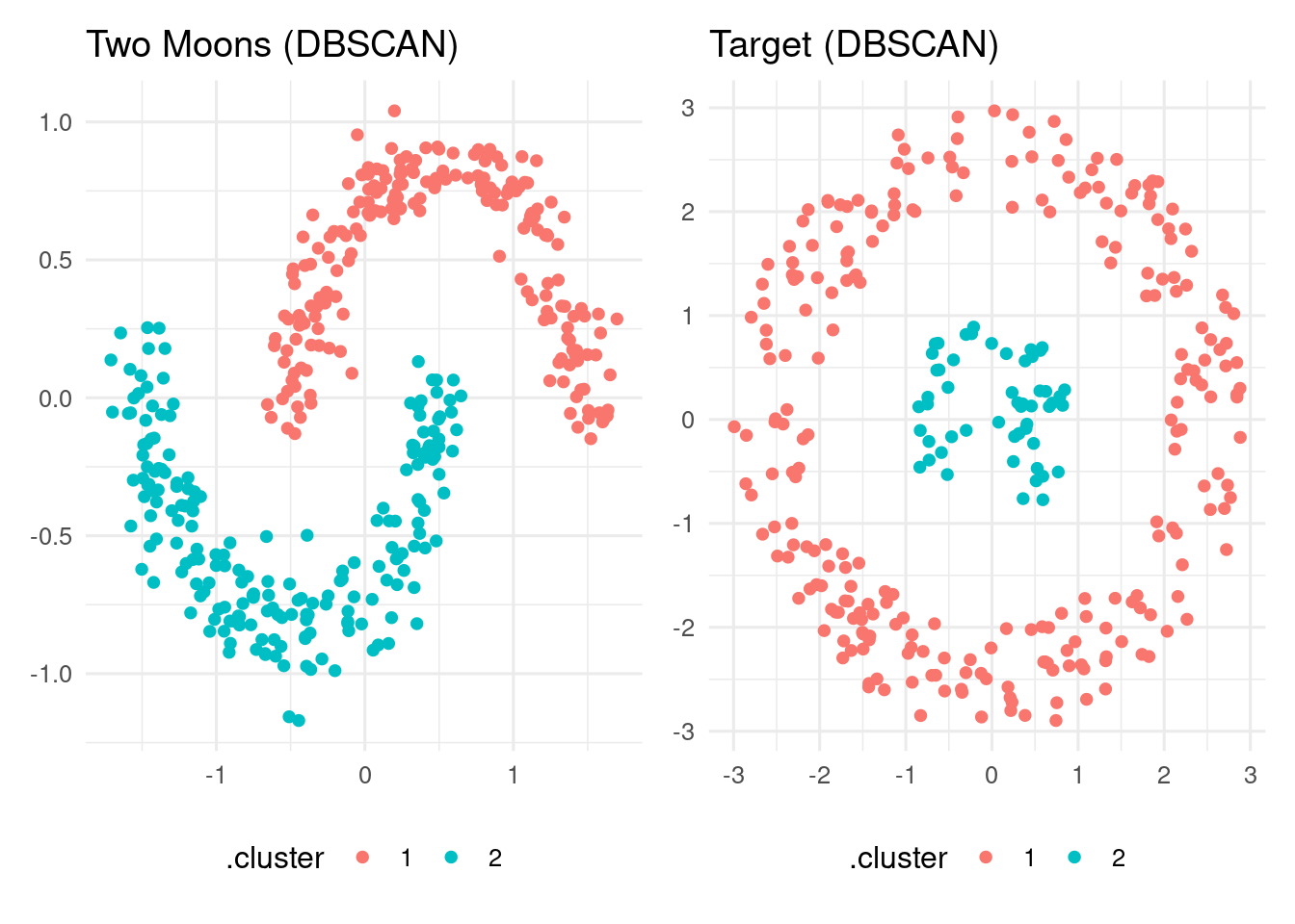

In both datasets, DBSCAN finds the two clusters of points as irregular, dense regions of points.

The DBSCAN algorithm

DBSCAN is a clustering algorithm that detects clusters as sets of points within regions denser than in the rest of the space. The algorithm relies on two parameters: the maximum distance between points eps and the minimum number of points reached by a core point minPts. In two-dimensional datasets is usual to set minPts = 3. The value of eps depends on the distance scale, and can be adjusted by trial and error. Large values of eps will produce few, large clusters and small values of eps many, small clusters.

DBSCAN is implemented in R with the dbscan package. As with R base clustering functions like kmeans() and hclust(), we can use the broom functions to obtain the output of the algorithm.

References

DBSCAN Wikipedia article: https://en.wikipedia.org/wiki/DBSCAN
Ester, Martin, Hans-Peter Kriegel, Jörg Sander, Xiaowei Xu, et al. (1996). A Density-Based Algorithm for Discovering Clusters in Large Spatial Databases with Noise. In Proceedings of 2nd International Conference on Knowledge Discovery and Data Mining (KDD-96), 226–231. https://dl.acm.org/doi/10.5555/3001460.3001507
fdm2id package: https://cran.r-project.org/web/packages/fdm2id/refman/fdm2id.html

Session Info

The package fdm2id has not been loaded. The two datasets have been loaded from an .rd file.

## R version 4.5.2 (2025-10-31)
## Platform: x86_64-pc-linux-gnu
## Running under: Linux Mint 21.1
## 
## Matrix products: default
## BLAS:   /usr/lib/x86_64-linux-gnu/blas/libblas.so.3.10.0 
## LAPACK: /usr/lib/x86_64-linux-gnu/lapack/liblapack.so.3.10.0  LAPACK version 3.10.0
## 
## locale:
##  [1] LC_CTYPE=es_ES.UTF-8       LC_NUMERIC=C              
##  [3] LC_TIME=es_ES.UTF-8        LC_COLLATE=es_ES.UTF-8    
##  [5] LC_MONETARY=es_ES.UTF-8    LC_MESSAGES=es_ES.UTF-8   
##  [7] LC_PAPER=es_ES.UTF-8       LC_NAME=C                 
##  [9] LC_ADDRESS=C               LC_TELEPHONE=C            
## [11] LC_MEASUREMENT=es_ES.UTF-8 LC_IDENTIFICATION=C       
## 
## time zone: Europe/Madrid
## tzcode source: system (glibc)
## 
## attached base packages:
## [1] stats     graphics  grDevices utils     datasets  methods   base     
## 
## other attached packages:
##  [1] patchwork_1.3.0 dbscan_1.2.3    broom_1.0.10    lubridate_1.9.4
##  [5] forcats_1.0.1   stringr_1.6.0   dplyr_1.1.4     purrr_1.2.0    
##  [9] readr_2.1.5     tidyr_1.3.1     tibble_3.3.0    ggplot2_4.0.0  
## [13] tidyverse_2.0.0
## 
## loaded via a namespace (and not attached):
##  [1] gtable_0.3.6       jsonlite_2.0.0     compiler_4.5.2     Rcpp_1.1.0        
##  [5] tidyselect_1.2.1   jquerylib_0.1.4    scales_1.4.0       yaml_2.3.10       
##  [9] fastmap_1.2.0      R6_2.6.1           labeling_0.4.3     generics_0.1.3    
## [13] knitr_1.50         backports_1.5.0    bookdown_0.43      tzdb_0.5.0        
## [17] bslib_0.9.0        pillar_1.11.1      RColorBrewer_1.1-3 rlang_1.1.6       
## [21] stringi_1.8.7      cachem_1.1.0       xfun_0.52          sass_0.4.10       
## [25] S7_0.2.0           timechange_0.3.0   cli_3.6.4          withr_3.0.2       
## [29] magrittr_2.0.4     digest_0.6.37      grid_4.5.2         rstudioapi_0.17.1 
## [33] hms_1.1.4          lifecycle_1.0.4    vctrs_0.6.5        evaluate_1.0.3    
## [37] glue_1.8.0         farver_2.1.2       blogdown_1.21      rmarkdown_2.29    
## [41] tools_4.5.2        pkgconfig_2.0.3    htmltools_0.5.8.1

The Jose M Sallan static website