Hierarchical linear regression is a way to examine if a set of predictor variables explains a criterion variable, after accounting the effect of control variables. In this modelling framework, we build several linear regression models adding blocks of variables at each step. Comparing the outcomes of the regression models, we can determine if the new block of variables increases significantly the proportion of explained variance of the criterion.
I will introduce hierarchical linear regression with three examples:
- a first dataset where there is a spurious correlation between predictor and criterion,
- a second dataset where there is a true relationship between criterion and predictor
- and a third dataset taken from University of Virginia Library, that clarifies the distinction between predictor and criterion.
I will be using the text output of the stargazer package to present the results of hierarchical linear regression models.
First dataset
Let’s build a set of artificial data to explain why we should be accounting for the effect of variables unrelated to the model:
n <- 100
con <- sample(25:45, n, replace = TRUE)
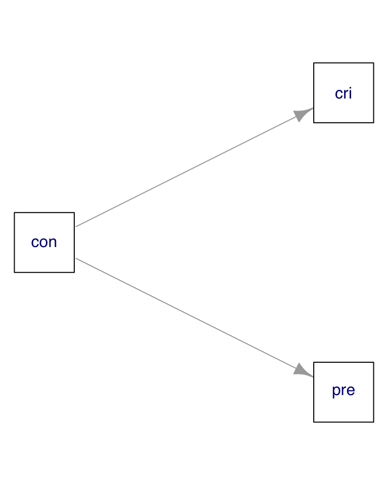
data01 <- data.frame(cri = 4 + 2*con + rnorm(n, mean = 0, sd = 2),
pre = 3 + con + rnorm(n, mean = 0, sd = 4),
con = con)
mod01 <- lm(cri ~ pre, data01)In the data01 dataset, the presumed predictor and criterion variables depend jointly on the control variable:
We cannot detect that if we examine the correlation matrix:
cor(data01)## cri pre con
## cri 1.0000000 0.8419584 0.9826853
## pre 0.8419584 1.0000000 0.8451160
## con 0.9826853 0.8451160 1.0000000We observe a strong correlation between criterion and predictor. This is not desirable, because ideally regressors must be uncorrelated. If we ignore this warning and naively regress the criterion on the predictor, we obtain a significant relationship between both variables, which does not exist:
mod01 <- lm(cri ~ pre, data = data01)
stargazer(mod01, type = "text")
##
## ===============================================
## Dependent variable:
## ---------------------------
## cri
## -----------------------------------------------
## pre 1.429***
## (0.093)
##
## Constant 19.042***
## (3.637)
##
## -----------------------------------------------
## Observations 100
## R2 0.709
## Adjusted R2 0.706
## Residual Std. Error 6.164 (df = 98)
## F Statistic 238.647*** (df = 1; 98)
## ===============================================
## Note: *p<0.1; **p<0.05; ***p<0.01To avoid this pitfall, we can adopt a hierarchical linear regression modelin framework with two models:
- a first model
mod01awhere we regress the criterion on the control variables - and a second model
mod01bwhere we regress the criterion on the control and predictor variables.
mod01a <- lm(cri ~ con, data01)
mod01b <- lm(cri ~ con + pre, data01)
I use the stargazer package to present both models together:
stargazer(mod01a, mod01b, type = "text")##
## =======================================================================
## Dependent variable:
## ---------------------------------------------------
## cri
## (1) (2)
## -----------------------------------------------------------------------
## con 1.956*** 1.889***
## (0.037) (0.070)
##
## pre 0.068
## (0.059)
##
## Constant 5.288*** 5.035***
## (1.334) (1.350)
##
## -----------------------------------------------------------------------
## Observations 100 100
## R2 0.966 0.966
## Adjusted R2 0.965 0.965
## Residual Std. Error 2.117 (df = 98) 2.113 (df = 97)
## F Statistic 2,756.677*** (df = 1; 98) 1,383.495*** (df = 2; 97)
## =======================================================================
## Note: *p<0.1; **p<0.05; ***p<0.01Now we observe that the coefficient of the predictor variable is not signiificant when we put it together with the control variable. We also observe that the coefficient of the control variable does not change significantly when we introduce the predictor. We conclude that the criterion does not depend on the predictor.
If we look at the R-square of both models, we learn that the second model is not better than the first. In fact, the adjusted R-square of the second model is worse than the first. Additionnaly, we can test the null hypothesis that the second model is not better than the first using the anova function:
anova(mod01a, mod01b)## Analysis of Variance Table
##
## Model 1: cri ~ con
## Model 2: cri ~ con + pre
## Res.Df RSS Df Sum of Sq F Pr(>F)
## 1 98 439.15
## 2 97 433.25 1 5.8945 1.3197 0.2535The low p-value makes us think that there are no sound reasons to discard the null hypothesis in this case.
Second dataset
Let’s build a new dataset, where the criterion variable depends on the predictor and control variables:
pre <- runif(n, 20, 100)
data02 <- data.frame(cri = 4 + 2*pre + 3*con + rnorm(n, mean = 0, sd = 10),
                     pre = pre,
                     con = con)
For this dataset, we know that the existing relationships are:
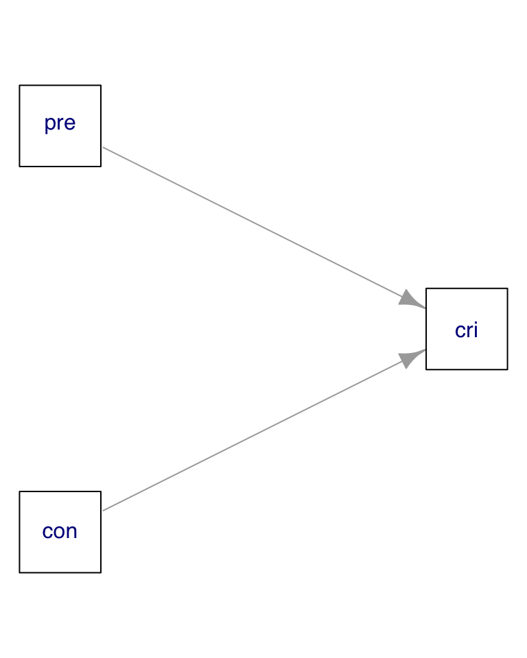
Now we observe a lower correlation between predictor and control, and a strong correlation between criterion and predictor:
cor(data02)## cri pre con
## cri 1.0000000 0.91792257 0.28037844
## pre 0.9179226 1.00000000 -0.06939176
## con 0.2803784 -0.06939176 1.00000000Let’s build the two models for the hierarchical linear regression, and present the results:
mod02a <- lm(cri ~ con, data02)
mod02b <- lm(cri ~ con + pre, data02)
stargazer(mod02a, mod02b, type = "text")
##
## ===================================================================
## Dependent variable:
## -----------------------------------------------
## cri
## (1) (2)
## -------------------------------------------------------------------
## con 2.384*** 2.940***
## (0.824) (0.170)
##
## pre 1.989***
## (0.042)
##
## Constant 136.114*** 6.860
## (29.512) (6.650)
##
## -------------------------------------------------------------------
## Observations 100 100
## R2 0.079 0.962
## Adjusted R2 0.069 0.961
## Residual Std. Error 46.847 (df = 98) 9.620 (df = 97)
## F Statistic 8.361*** (df = 1; 98) 1,212.618*** (df = 2; 97)
## ===================================================================
## Note: *p<0.1; **p<0.05; ***p<0.01Now the coefficient of the predictor variable is significant, when put together with the control variable. We also observe that the coefficient of the control variable keeps being significant in the second model. We observe a significant increase of the R-square of the second model respect to the first. Finnally, we also observe that the anova test is significant:
anova(mod02a, mod02b)## Analysis of Variance Table
##
## Model 1: cri ~ con
## Model 2: cri ~ con + pre
## Res.Df RSS Df Sum of Sq F Pr(>F)
## 1 98 215073
## 2 97 8977 1 206096 2227 < 2.2e-16 ***
## ---
## Signif. codes: 0 '***' 0.001 '**' 0.01 '*' 0.05 '.' 0.1 ' ' 1Now we can conclude that there is a significant relationship between predictor and criterion, after controlling by control variables.
Third dataset
Let’s perform now hierarchical regression on a dataset with five variables, obtained from the University of Virginia Library:
happiness_data <- read.csv('http://static.lib.virginia.edu/statlab/materials/data/hierarchicalRegressionData.csv')
head(happiness_data)
## happiness age gender friends pets
## 1 5 24 Male 12 3
## 2 5 28 Male 8 1
## 3 6 25 Female 6 0
## 4 4 26 Male 4 2
## 5 3 20 Female 8 0
## 6 5 25 Male 9 0Our aim is to determine if happiness increases when we have more friends and more pets, controlling by age and gender. By controlling by this demographic variables, we rid out the possibility that happinness and number of friends or pets depend on age or gender.
Let’s examine first the correlation matrix between numerical variables. We observe a low correlation between controls and predictors:
cor(happiness_data[, c(1:2, 4:5)])## happiness age friends pets
## happiness 1.0000000 -0.16091772 0.32424344 0.29948447
## age -0.1609177 1.00000000 -0.02097324 -0.03786638
## friends 0.3242434 -0.02097324 1.00000000 0.11941881
## pets 0.2994845 -0.03786638 0.11941881 1.00000000And let’s examine the result of the hierarchical linear regression model:
hmod01 <- lm(happiness ~ age + gender, data=happiness_data)
hmod02 <- lm(happiness ~ age + gender + friends + pets, data=happiness_data)
stargazer(hmod01, hmod02, type = "text")
##
## ============================================================
## Dependent variable:
## ----------------------------------------
## happiness
## (1) (2)
## ------------------------------------------------------------
## age -0.130 -0.111
## (0.079) (0.073)
##
## genderMale 0.164 -0.143
## (0.319) (0.312)
##
## friends 0.171***
## (0.055)
##
## pets 0.364***
## (0.130)
##
## Constant 7.668*** 5.785***
## (2.014) (1.903)
##
## ------------------------------------------------------------
## Observations 100 100
## R2 0.029 0.197
## Adjusted R2 0.009 0.163
## Residual Std. Error 1.553 (df = 97) 1.427 (df = 95)
## F Statistic 1.425 (df = 2; 97) 5.822*** (df = 4; 95)
## ============================================================
## Note: *p<0.1; **p<0.05; ***p<0.01Here we observe that:
- The status of the coefficients of the two control variables does not change when we add the predictor variables
- The coefficients of the two predictor variables are significant and positive.
Additionally, the ANOVA between the two models is significant:
anova(hmod01, hmod02)## Analysis of Variance Table
##
## Model 1: happiness ~ age + gender
## Model 2: happiness ~ age + gender + friends + pets
## Res.Df RSS Df Sum of Sq F Pr(>F)
## 1 97 233.97
## 2 95 193.42 2 40.542 9.9561 0.0001187 ***
## ---
## Signif. codes: 0 '***' 0.001 '**' 0.01 '*' 0.05 '.' 0.1 ' ' 1From that analysis we conclude that happiness is positively related with number of friends and number of pets, after controlling by gender and age.
Observing the effect of predictors with hierarchical linear regression
We can conclude that a relationship between a criterion and a set of predictor variables exists, after controlling by a set of control variables, if the following conditions hold:
- The status of the coefficients of the control variables does not change after adding the predictors.
- The explanatory power of the model with predictors and controls (second model) is higher than the model with controls alone (first model). By can check that examining the change of R-squared, which must be significantly higher for the second model. We can also perform an ANOVA test on both models, to discard the null hypothesis that the second model explains the same variance of the criterion variable as the first.
References
- Hierarchical Linear Regression (University of Virginia Library) https://data.library.virginia.edu/hierarchical-linear-regression/
stargazercheatsheet https://www.jakeruss.com/cheatsheets/stargazer/
Built with R 4.1.0, stargazer 5.2.2 and igraph 1.2.6